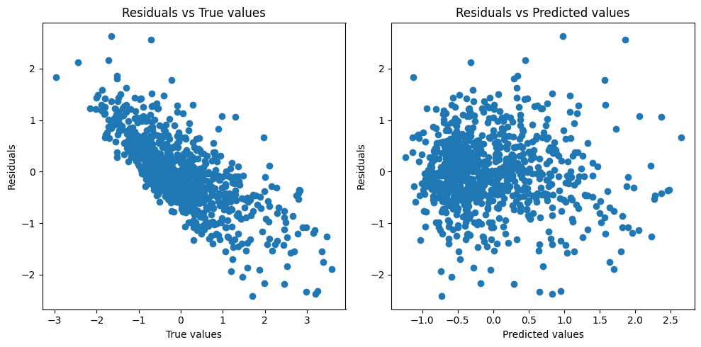
I built a neural network using PyTorch to predict y (a continuous variable) based on X consisting of m (=20) features. I found that the residuals (y_predicted – y_true) for the test data set show a clear linear trend with the true value ‘y_ture’ .
In addition, I can observe a linear relation between y_predicted and y_true, with R2 equal to about 0.5. Another observation is that the model tends to overestimate lower values of y but underestimate larger values of y, leading to the value range of the predicted y is evidently smaller than that of the true values.
I have tried the following ways to avoid the linear trend in the residuals: 1) increased the complexity of the model, by increasing the number of hidden layers and neurons for hidden layers, 2) added dropout scheme, early-stopping criterion, and regularization term to avoid overfitting. But they did not work, and the linear trend still exists. I also tried to design a network that incorporates an additional component to learn the linear trend and added the predicted error back to the predicted value of y, but I did not know how to design it effectively. Is there anyone who can help me to remove the linear trend in the residuals and further enhance the model?
    import torch
    import torch.nn as nn
    import torch.optim as optim
    from torch.utils.data import Dataset, DataLoader
    import numpy as np
    from sklearn.model_selection import train_test_split
    from sklearn.metrics import r2_score
    import matplotlib.pyplot as plt

    # Define the custom dataset
    class CustomDataset(Dataset):
        def __init__(self, X, y):
            self.X = torch.FloatTensor(X)
            self.y = torch.FloatTensor(y).reshape(-1, 1)

        def __len__(self):
            return len(self.y)

        def __getitem__(self, idx):
            return self.X[idx], self.y[idx]

    # Define the neural network
    class NeuralNetwork(nn.Module):
        def __init__(self, input_size):
            super(NeuralNetwork, self).__init__()
            self.layers = nn.Sequential(
                nn.Linear(input_size, 64),
                nn.ReLU(),
                nn.Dropout(0.2),
                nn.Linear(64, 32),
                nn.ReLU(),
                nn.Dropout(0.2),
                nn.Linear(32, 16),
                nn.ReLU(),
                nn.Dropout(0.2),
                nn.Linear(16, 1)
            )

        def forward(self, x):
            return self.layers(x)

    # Function to train the model
    def train_model(model, train_loader, val_loader, criterion, optimizer, num_epochs, patience):
        best_val_loss = float('inf')
        epochs_no_improve = 0

        for epoch in range(num_epochs):
            model.train()
            for inputs, targets in train_loader:
                optimizer.zero_grad()
                outputs = model(inputs)
                loss = criterion(outputs, targets)
                loss.backward()
                optimizer.step()

            # Validation
            model.eval()
            val_loss = 0
            with torch.no_grad():
                for inputs, targets in val_loader:
                    outputs = model(inputs)
                    val_loss += criterion(outputs, targets).item()

            val_loss /= len(val_loader)

            if val_loss < best_val_loss:
                best_val_loss = val_loss
                epochs_no_improve = 0
                torch.save(model.state_dict(), 'best_model.pth')
            else:
                epochs_no_improve += 1

            if epochs_no_improve == patience:
                print(f"Early stopping triggered after {epoch + 1} epochs")
                break

        model.load_state_dict(torch.load('best_model.pth'))
        return model

    # Function to evaluate the model
    def evaluate_model(model, test_loader):
        model.eval()
        predictions = []
        actuals = []
        with torch.no_grad():
            for inputs, targets in test_loader:
                outputs = model(inputs)
                predictions.extend(outputs.numpy().flatten())
                actuals.extend(targets.numpy().flatten())

        r2 = r2_score(actuals, predictions)
        return r2, predictions, actuals

    # Function to plot residuals
    def plot_residuals(y_true, y_pred):
        residuals = y_pred - y_true
        plt.figure(figsize=(10, 5))

        plt.subplot(1, 2, 1)
        plt.scatter(y_true, residuals)
        plt.xlabel('True values')
        plt.ylabel('Residuals')
        plt.title('Residuals vs True values')

        plt.subplot(1, 2, 2)
        plt.scatter(y_pred, residuals)
        plt.xlabel('Predicted values')
        plt.ylabel('Residuals')
        plt.title('Residuals vs Predicted values')

        plt.tight_layout()
        plt.show()

    # Main execution
    def main():
        # Assuming you have your data in X and y
        # X = ... # Your input data (n_samples, 20)
        # y = ... # Your target data (n_samples,)

        # Split the data
        X_train, X_test, y_train, y_test = train_test_split(X, y, test_size=0.2, random_state=42)
        X_train, X_val, y_train, y_val = train_test_split(X_train, y_train, test_size=0.2,             random_state=42)

        # Create datasets and dataloaders
        train_dataset = CustomDataset(X_train, y_train)
        val_dataset = CustomDataset(X_val, y_val)
        test_dataset = CustomDataset(X_test, y_test)

        train_loader = DataLoader(train_dataset, batch_size=32, shuffle=True)
        val_loader = DataLoader(val_dataset, batch_size=32)
        test_loader = DataLoader(test_dataset, batch_size=32)

        # Initialize the model
        model = NeuralNetwork(input_size=20)

        # Define loss function and optimizer
        criterion = nn.MSELoss()
        optimizer = optim.Adam(model.parameters(), lr=0.001, weight_decay=1e-5)  # L2 regularization

        # Train the model
        model = train_model(model, train_loader, val_loader, criterion, optimizer, num_epochs=100, patience=10)

        # Evaluate the model
        r2, predictions, actuals = evaluate_model(model, test_loader)
        print(f"R2 score on test set: {r2}")

        # Plot residuals
        plot_residuals(np.array(actuals), np.array(predictions))

    if __name__ == "__main__":
        main()
This is the resulting figure:

