Survival analysis for survey (case-control?) data

Question

I have a dataset comprising approximately 500 patients with about 10 different diseases, potentially with correlated outcomes, and 200 healthy controls. Patient data is sourced from the hospital, while control data comes from volunteers and is not matched. We have comprehensive records of various life events, including specific dates (e.g., age of first-time illegal drug use) and dates of diagnosis for both patients and controls. However, no sampling weights are available.

As a first step, I plan to apply a Cox proportional hazards (PH) model to each disease individually, using birth as the time reference (time = 0). The events are binary (whether a disease is diagnosed or not). The dataset includes around 10 potential predictors, such as sex, race, and education, with some covariates potentially being time-dependent (e.g., marriage history and employment).

(A) Given that cases are oversampled, can I weight the sample based on prevalence or incidence rates from external sources? (A link of previous papers doing this will be extremely helpful.).

(B) Can this study be considered a case-cohort study, even though it does not fit the traditional definition?

(C) While logistic regression is typically used for case-control studies (yielding only odds ratios), is there an analogous approach in survival analysis for dealing with this type of data?

Thank you!

Answer 1

The answer from Sextus Empiricus (+1) gets to a major issue that you raised, whether you could use something like case-cohort analysis for your study. You can't.

Second, you seem to want to be able to extend the results of your Cox proportional hazards regression to a broader, more representative population. There are more issues with that than can be explained here, even for a descriptive model that doesn't attempt to get at causal inference. Chapter 10 of Therneau and Grambsch discusses many of those issues, based on the implicit assumption that your model is correct.

There are additional issues with your study design that need to be addressed.

Left truncation. Unless you have information on all individuals available since the date of birth, your time values are necessarily left truncated. For example, someone for whom you have the first data at an age of 27 provides no information about those in the population at younger ages.

Although that's nicely handled by the counting-process data format that you will presumably be using for time-varying covariates (the start time for each time intervals is treated as a left truncation), with the time = 0 reference at birth you probably will have very little information about young ages. Klein and Moeschberger discuss that problem in Section 4.6. In practice, you might have to analyze data conditional upon having survived to some age at which you have enough data to be useful.

An analog to odds ratios. I think this is implicit in the answer from Sextus Empiricus, but I'll but put it in my own words. As you recognize, logistic regression coefficients can provide useful information about odds ratios associated with a difference in predictor values, even when the intercept can't be generalized to the population (as in a case-control study).

The analog in a Cox proportional hazard model is the hazard ratio, the relative event hazard associated with a difference in predictor values. Insofar as you have a valid model those hazard ratios will provide similarly useful information. The analog to the intercept of a logistic regression model in such a model is the entire baseline survival curve, which can be estimated once the Cox model is fit but which has discrete steps at the observed event times and might only apply to the population that was sampled.

Volunteers as controls. Hernán and Robins show that relying on volunteers can risk selection bias (Section 8.2).* If your cases were from all those in your records having these diseases while your controls were all volunteers, that might be a problem.

Covariates. If you don't use some form of penalization, then you typically need about 15 events (not individuals) per coefficient that you are estimating in a survival regression. If you want to evaluate 10 predictors in a model for a single disease, you would thus need about 150 individuals with the disease. But if you cut down the number of predictors and omit an outcome-associated predictor from a Cox model you risk omitted-variable bias. See Frank Harrell's Regression Modeling Strategies for general background, in particular Chapter 4 for this issue and principled data-reduction approaches to cut down on the (effective) number of predictors.

Time-varying covariates. If you use time-varying covariates, recognize that a Cox model only evaluates the instantaneous values among those at risk at each event time, not any history of the values (unless you define a new covariate related to that history).

Multiple diseases. You recognize that the 10 diseases might be correlated. Individual models for each disease won't handle that and will also lead to a multiple comparisons problem. A multi-state model might be preferable, treating each disease as a separate type of event.

I strongly recommend that you consult with a statistician having experience in survival analysis, to see what you might be able to glean reliably from such a study.

---

*That reference is a valuable introduction to the problems of moving beyond simple description of data to causal inference. Chapter 17 is specifically on causal survival analysis, and the last 5 chapters deal with the problems associated with time-varying treatments.

Answer 2

Here is an explanation of the mathematics behind a case-cohort study.

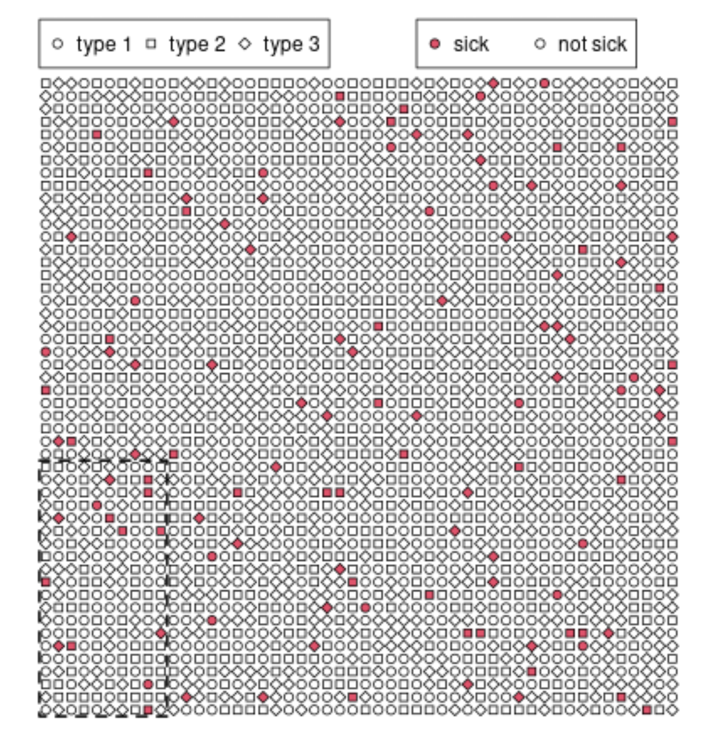
Below we see a sketch for a simulation of data in a cohort study among 2500 people with an 'outcome' sick vs not sick and this is being studied as a function of a variable 'type' which has 3 levels.

If we study the entire cohort then we would have a contingency table like

$$\begin{array}{r|ccc} &\text{type 1}&\text{ type 2}&\text{ type 3} \\ \hline \text{sick}&19&43&54 \\ \text{not sick}&840&798&746\\ \\ \text{sum}&859&841&800\\ \end{array}$$

This requires to measure the types among all 2500 patients.

The alternative with a case-cohort study is to have a sub-cohort like the 200 people in the 10 by 20 square in the lower left corner and only determine the types in the sub cohort and the positive cases. Then the table will look like:

$$\begin{array}{r|ccc|ccc} &\rlap{\text{rest of cohort}}&&&\rlap{\text{sub cohort}}\\ &\text{type 1}&\text{ type 2}&\text{ type 3} &\text{type 1}&\text{ type 2}&\text{ type 3} \\ \hline \text{sick}&17&35&50 &2&8&4\\ \text{not sick}&\color{pink}{768}&\color{pink}{732}&\color{pink}{698}&72&66&48\\ \\ \text{sum}&\color{pink}{785}&\color{pink}{767}&\color{pink}{748}&74&74&52\\ \end{array}$$

Here, the pink numbers are not observed. And we only know the 12 data values in black.

These values can be modelled based on the probabilities of the disease occuring or not for the types, $p_1,p_2,p_3$, as well as the odds of being outside the sub-cohort $o_{\neg sub}$ and the numbers in the subcohort $n_1,n_2,n_3$.

$$\begin{array}{r|ccc|ccc} &\rlap{\text{rest of cohort}}&&&\rlap{\text{sub cohort}}\\ &\text{type 1}&\text{ type 2}&\text{ type 3} &\text{type 1}&\text{ type 2}&\text{ type 3} \\ \hline \text{sick}&p_1n_1o_{\neg sub}&p_2n_2o_{\neg sub}&p_3n_3o_{\neg sub} &p_1n_1&p_2n_2&p_3n_3 \\ \text{not sick}&-&-&-&(1-p_1)n_1&(1-p_2)n_2&(1-p_3)n_3 \\ \hline \text{total}&-&-&-&n_1&n_2&n_3 \end{array}$$

The above is the case for a contingency table, the same may be done for a proportional hazards model. Now the computations are potentially not including those bins anymore (e.g. if the variables are continuous instead of categorical), but then we have all the $n_i=1$ and it works the same. For a relative hazards model, you compute the odds of occuring in a specific individual given that somebody got sick, and you see that there is an additional factor $o_{\neg sub}$ if that individual is outside the sub-cohort.

---

• (A)

  can I weight the sample based on prevalence or incidence rates from external sources?

  The weighing occurs based on the odds of being in the sub-cohort.

• (B)

  Can this study be considered a case-cohort study?

  The case-cohort study selects a sub-cohort that is independent from being sick or not. Your controls may have been selected depending on whether they are not sick. Possibly you may perform some similar corrections but it is not the same. You can not make the 2nd table like above where you can compute the prevalences of the types, and you can not make the step from contingency to proportional hazards in case of continuous variables (where there are no categories and no clearly defined prevalences).

• (C)

  is there an analogous approach in survival analysis

  Because it is simpler, I have made an example with a contingency table. So that is one analogous approach. The problem with this alternative is that it doesn't work with continuous variables and with variable exposure times among subjects.

  Beyond that, there are many others. Any alternative to relative hazards (e.g. an accelerated time model) can give an analogues approach. You just add the factor $o_{\neg sub}$ for the risk.

---

Code for image

set.seed(1)

n = 50
type = sample(1:3, n^2, replace = TRUE)
x = rep(1:n,n)
y = rep(1:n,each=n)
p = type/50
sick = rbinom(n^2,1,p)

par(mar = c(1,1,1,1))
plot(x,y,pch=20+type, cex = 1,
     xlab = "", ylab = "",
     xaxt = "n", yaxt = "n",
     bg = 0+2*sick, bty = "n", xlim = c(0,n+5), ylim = c(0,n+5))

legend(0.5,n+5, c("type 1", "type 2", "type 3"), pch = c(21,22,23), ncol = 3)

legend(30,n+5, c("sick", "not sick"), pt.bg = c(2,0), pch = 21, ncol = 2)

lines(c(0,10,10,0,0)+0.5,
      c(20,20,0,0,20)+0.5, lty = 2, lwd = 2)

sub = (x<=10)*(y<=20)

table(sick, paste0(sub,type))
table(sick, paste0(type))  

Answer 3

I think you can just build binary classifiers to build your discrete-time survival model: https://bmcmedresmethodol.biomedcentral.com/articles/10.1186/s12874-022-01679-6 See especially the discussion around figure 1) to understand how you need to resample your data for a discrete-time survival model

This approach is super flexible. I miss the discussion of discrete-time survival models a lot! For a calibrated classifier the predicted score is the hazard probability in a given time interval.

Additionally proper scoring rules and the evaluation metrics of a binary classifier help you judge your model's predictive performance (on hold out test sets)

For your question A) yes: if you know your samples are not drawn according to the population distribution (but are oversampled), you could take care of this when constructing the training set for the classifier - you would then draw samples from the oversampled survival times less frequently.

Some main take-aways from the paper of Krithika Suresh, Cameron Severn & Debashis Ghosh:

• "Note that we do not make the assumption that the event indicators within a subject are independent and have a binomial distribution. Instead, we observe that the likelihood function for the discrete-time survival model under non-informative censoring can be represented using a binomial likelihood that assumes independent event indicators"

• "Due to the binomial structure of the likelihood function in Eq. (2) the discrete survival time formulation is general and any algorithm that can optimize a binomial log-likelihood can be used to obtain parameter estimates. Thus, within this approach we can apply any method for computing the probability of a binary event and can choose from various binary classification methods, from traditional regression methods to more complex machine learning approaches."