Discrepancy in MSE Cell Frequencies and Entropy Estimation for Various Estimators

Question

I've been trying to replicate the results from the paper "Entropy Inference and the James-Stein Estimator, With Application to Nonlinear Gene Association Networks" in R. The goal is to compare different entropy estimators across multiple scenarios. I've implemented the estimators, including Maximum Likelihood, Miller-Madow, various Bayesian approaches, Chao-Shen, and a Shrinkage estimator.

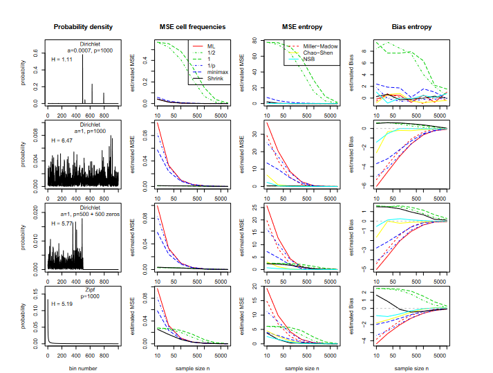
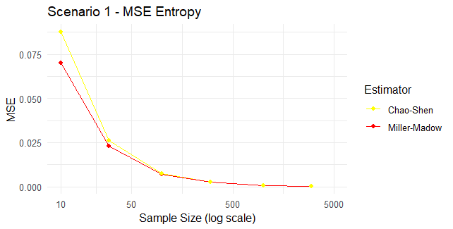
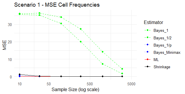
While the general trends in the plots for MSE Cell Frequencies and MSE Entropy seem similar to those presented in the paper, the specific values on the axes are significantly different from what is reported in the paper. I've tried various tweaks and double-checked my implementation, but the issue persists.

Here is a summary of what I've done:

1. Generated Data: Using a Dirichlet distribution with different parameterizations to simulate the scenarios described in the paper (small alpha, alpha=1, half-zero probabilities, and Zipf distribution).
2. Implemented Entropy Estimators: Including the Maximum Likelihood (ML), Miller-Madow, Bayesian with different priors, Chao-Shen, and Shrinkage (James-Stein) estimators.
3. Calculated MSE and Bias: For each sample size, I computed the Mean Squared Error (MSE) for the entropy estimates compared to the true entropy.
4. Plotted the Results: I've created plots for MSE Cell Frequencies, MSE Entropy across different sample sizes.

The plots look similar in shape to those in the paper but are off in terms of axis values. For example, the MSE values for the different estimators are much higher than expected.

Screenshots of the Plots:

Our Final goal should look like this (See the first row):

(I'm aware that are missing some estimator missing in the MSE Entropy, I'll add them soon)

Here is a snippet of my code where I calculate the MSE:

# Load libraries
library(gtools)
library(ggplot2)
library(entropy)
library(gridExtra)

# Shannon Entropy
shannon_entropy <- function(probabilities) {
  -sum(probabilities * log(probabilities + 1e-10))
}

# Maximum Likelihood Estimator
entropy_ml <- function(counts) {
  probabilities <- counts / sum(counts)
  shannon_entropy(probabilities)
}

# Miller-Madow Estimator
entropy_miller_madow <- function(counts) {
  n <- sum(counts)
  m_pos <- sum(counts > 0)
  entropy_ml(counts) + (m_pos - 1) / (2 * n)
}

# Bayesian Estimators with different priors
entropy_bayes <- function(counts, a) {
  n <- sum(counts)
  A <- sum(a)
  theta_bayes <- (counts + a) / (n + A)
  shannon_entropy(theta_bayes)
}

# Chao-Shen Estimator
entropy_chao_shen <- function(counts) {
  entropy.ChaoShen(counts)
}

# Shrinkage Estimator (James-Stein)
entropy_shrinkage <- function(counts) {
  entropy.shrink(counts)
}

# Function to Generate Data
generate_data <- function(p, sample_size, scenario) {
  if (scenario == 1) {
    alpha <- rep(0.0007, p)
    true_probs <- rdirichlet(1, alpha)
  } else if (scenario == 2) {
    alpha <- rep(1, p)
    true_probs <- rdirichlet(1, alpha)
  } else if (scenario == 3) {
    alpha <- rep(1, p)
    true_probs <- rdirichlet(1, alpha)
    true_probs[1:(p/2)] <- 0
    true_probs <- true_probs / sum(true_probs)
  } else if (scenario == 4) {
    zipf_probs <- 1 / (1:p)
    true_probs <- zipf_probs / sum(zipf_probs)
  } else {
    stop("Invalid scenario")
  }
  
  counts <- rmultinom(1, size = sample_size, prob = true_probs)
  list(true_probs = true_probs, counts = as.vector(counts))
}

# Function to Calculate MSE and Bias
calculate_mse_bias <- function(counts, true_probs) {
  true_entropy <- shannon_entropy(true_probs)
  
  # Entropy estimates
  entropy_estimates <- c(
    ML = entropy_ml(counts),
    MillerMadow = entropy_miller_madow(counts),
    Bayes_1 = entropy_bayes(counts, rep(1, length(counts))),
    Bayes_1_2 = entropy_bayes(counts, rep(0.5, length(counts))),
    Bayes_Minimax = entropy_bayes(counts, sqrt(counts)),
    Bayes_1_p = entropy_bayes(counts, rep(1/length(counts), length(counts))),
    Chao_Shen = entropy_chao_shen(counts),
    Shrinkage = entropy_shrinkage(counts)
  )
  
  # MSE Entropy (comparing estimated entropy with true entropy)
  mse_entropy <- (entropy_estimates - true_entropy)^2
  
  return(list(mse_entropy = mse_entropy))
}

# Simulation Parameters
p <- 1000
sample_sizes <- c(10, 30, 100, 300, 1000, 3000, 10000)
scenarios <- 1:4
n_simulations <- 1000

# Initialize Results Storage
results_list <- list()



for (scenario in scenarios) {
  for (sample_size in sample_sizes) {
    mse_list <- list()
    
    entropy_estimates <- matrix(NA, nrow = n_simulations, ncol = 8)
    colnames(entropy_estimates) <- c(
      "ML", "Miller-Madow", "Bayes_1", "Bayes_1/2", 
      "Bayes_Minimax", "Bayes_1/p", "Chao-Shen", "Shrinkage"
    )
    
    valid_simulations <- 0
    attempts <- 0
    max_attempts <- n_simulations * 2
    
    while (valid_simulations < n_simulations && attempts < max_attempts) {
      attempts <- attempts + 1
      data <- generate_data(p, sample_size, scenario)
      counts <- data$counts
      true_probs <- data$true_probs
      true_entropy <- shannon_entropy(true_probs)
      
      if (sum(counts > 0) >= 2) {
        valid_simulations <- valid_simulations + 1
        
        true_entropy <- shannon_entropy(true_probs)
        
        # Calculate MSE and Bias for this simulation
        mse_bias <- calculate_mse_bias(counts, true_probs)
        
        entropy_estimates[valid_simulations, ] <- mse_bias$mse_entropy
      }
    }
    
    if (valid_simulations < n_simulations) {
      warning(paste(
        "Could not generate enough valid simulations for Scenario", scenario, 
        "and Sample Size", sample_size
      ))
      next
    }
    
    mse <- colMeans(entropy_estimates, na.rm = TRUE)
    bias <- colMeans(entropy_estimates - true_entropy, na.rm = TRUE)
    
    results_list[[paste(
      "Scenario", scenario, "SampleSize", sample_size, sep = "_"
    )]] <- list(
      mse = mse,
      bias = bias,
      true_probs = data$true_probs,
      counts = counts
    )
  }
}


# Prepare Data for Plotting
plot_data <- data.frame()

for (name in names(results_list)) {
  parts <- strsplit(name, "_")[[1]]
  scenario <- parts[2]
  sample_size <- as.numeric(parts[4])
  mse <- results_list[[name]]$mse
  bias <- results_list[[name]]$bias
  
  temp_data <- data.frame(
    Scenario = scenario,
    SampleSize = sample_size,
    Estimator = names(mse),
    MSE = as.numeric(mse),
    Bias = as.numeric(bias)
  )
  
  plot_data <- rbind(plot_data, temp_data)
}

# Descriptive scenario labels
scenario_labels <- c(
  "Scenario 1: Dirichlet with small alpha",
  "Scenario 2: Dirichlet with alpha=1",
  "Scenario 3: Dirichlet with half zeros",
  "Scenario 4: Zipf distribution"
)

## PLOTTING GALATTICO
generate_plots <- function(scenario, plot_data) {
  scenario_label <- scenario_labels[as.character(scenario)]
  scenario_pattern <- paste0("Scenario_", scenario, "_")
  scenario_data <- results_list[grep(scenario_pattern, names(results_list))]
  
  if (length(scenario_data) == 0) {
    stop(paste("No data available for Scenario", scenario))
  }
  
  largest_sample_size_data <- scenario_data[[length(scenario_data)]]
  filtered_probs <- largest_sample_size_data$true_probs[largest_sample_size_data$true_probs > 1e-10]
  
  # Probability Density Plot
  prob_density_plot <- ggplot(data = data.frame(bin_number = 1:length(filtered_probs), probability = filtered_probs), 
                              aes(x = bin_number, y = probability)) +
    geom_bar(stat = "identity", color = "black", fill = "black") +
    labs(title = paste("Scenario", scenario, "- Probability Distribution (H =", round(shannon_entropy(filtered_probs), 2), ")"), 
         x = "Bin Number", y = "Probability") +
    theme_minimal() +
    theme(
      axis.title = element_text(size = 12),
      axis.text = element_text(size = 10),
      plot.title = element_text(size = 14, face = "bold")
    )
  
  # Define line types for specific estimators
  line_types <- c(
    "ML" = "solid",
    "Miller-Madow" = "solid",
    "Bayes_1" = "dashed",
    "Bayes_1/2" = "dashed",
    "Bayes_Minimax" = "dotted",
    "Bayes_1/p" = "dotted",
    "Chao-Shen" = "solid",
    "Shrinkage" = "solid"
  )
  
  # Filter out "Miller-Madow" and "Chao-Shen" for MSE Cell Frequencies Plot
  filtered_plot_data_mse_cell_frequencies <- plot_data[!plot_data$Estimator %in% c("Miller-Madow", "Chao-Shen"), ]
  
  # MSE Cell Frequencies Plot
  mse_cell_frequencies_plot <- ggplot(filtered_plot_data_mse_cell_frequencies[filtered_plot_data_mse_cell_frequencies$Scenario == scenario, ], 
                                      aes(x = SampleSize, y = MSE, color = Estimator, linetype = Estimator, group = Estimator)) +
    geom_line() +
    geom_point() +
    scale_x_log10(limits = c(10, 5000), breaks = c(10, 50, 500, 5000)) +
    scale_color_manual(values = c(
      "ML" = "red",
      "Miller-Madow" = "red",
      "Bayes_1" = "green",
      "Bayes_1/2" = "green",
      "Bayes_Minimax" = "blue",
      "Bayes_1/p" = "blue",
      "Chao-Shen" = "yellow",
      "Shrinkage" = "black"
    )) +
    scale_linetype_manual(values = line_types) +
    labs(title = paste("Scenario", scenario, "- MSE Cell Frequencies"), 
         x = "Sample Size (log scale)", y = "MSE") +
    theme_minimal()
  
  # Filter out "ML", "Bayes_1", "Bayes_1/2", "Bayes_Minimax", "Bayes_1/p" and "Shrinkage" for MSE Entropy plots
  filtered_plot_data_mse_entropy <- plot_data[plot_data$Estimator %in% c("Miller-Madow", "Chao-Shen"), ]
  
  # MSE Entropy Plot
  mse_entropy_plot <- ggplot(filtered_plot_data_mse_entropy[filtered_plot_data_mse_entropy$Scenario == scenario, ], 
                             aes(x = SampleSize, y = MSE, color = Estimator, linetype = Estimator, group = Estimator)) +
    geom_line() +
    geom_point() +
    scale_x_log10(limits = c(10, 5000), breaks = c(10, 50, 500, 5000)) +
    scale_color_manual(values = c(
      "ML" = "red",
      "Miller-Madow" = "red",
      "Bayes_1" = "green",
      "Bayes_1/2" = "green",
      "Bayes_Minimax" = "blue",
      "Bayes_1/p" = "blue",
      "Chao-Shen" = "yellow",
      "Shrinkage" = "black"
    )) +
    scale_linetype_manual(values = line_types) +
    labs(title = paste("Scenario", scenario, "- MSE Entropy"), 
         x = "Sample Size (log scale)", y = "MSE") +
    theme_minimal()
  
  # Bias Entropy Plot
  bias_entropy_plot <- ggplot(plot_data[plot_data$Scenario == scenario, ], 
                              aes(x = SampleSize, y = Bias, color = Estimator, linetype = Estimator, group = Estimator)) +
    geom_line() +
    geom_point() +
    scale_x_log10() +
    scale_color_manual(values = c(
      "ML" = "red",
      "Miller-Madow" = "red",
      "Bayes_1" = "green",
      "Bayes_1/2" = "green",
      "Bayes_Minimax" = "blue",
      "Bayes_1/p" = "blue",
      "Chao-Shen" = "yellow",
      "Shrinkage" = "black"
    )) +
    scale_linetype_manual(values = line_types) +
    labs(title = paste("Scenario", scenario, "- Bias Entropy"), 
         x = "Sample Size (log scale)", y = "Bias") +
    theme_minimal()
  
  return(list(
    prob_density_plot, 
    mse_cell_frequencies_plot, 
    mse_entropy_plot, 
    bias_entropy_plot
  ))
}


# Generate and Display Plots for Each Scenario
for (scenario in scenarios) {
  plots <- generate_plots(scenario, plot_data)
  for (plot in plots) {
    print(plot)
  }
}

NB: Ignore the Bias calculation parts, they are still a work in progress

Thank you for your help!