Inflated fixed effects in mixed-effects logistic regression model

Question

I have a dataset with multiple observations per ID and a binary outcome. I am trying to fit a mixed-effects logistic regression, however, the fixed effect estimate of the intercept is extremely large compared to what I would expect. This is true regardless of the statistical package or the R version I am using:

library(lme4)
library(glmmTMB)
library(brms)

fit_lme4 <-   glmer(outcome ~ (1 | ID), data = data, family = "binomial")
fit_TMB  <- glmmTMB(outcome ~ (1 | ID), data = data, family = "binomial")
fit_brm  <-     brm(outcome ~ (1 | ID), data = data, family = bernoulli(link="logit"))

mean(data$outcome)                  # 0.7371429
plogis(fixef(fit_lme4))             # 0.9993405
plogis(fixef(fit_lme4)$cond)        # 0.9993405
plogis(summary(fit_brm)$fixed[[1]]) # 0.9452537

Here is the content of data for reproducing the above script.

I suspect this may be because many IDs always have the same outcome (e.g., for ID 1, the outcome is always 1), but I am unsure.

What is a potential solution to this?

Answer 1

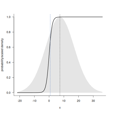
There's nothing wrong with your model. This is a combined consequence of very high among-ID variation and Jensen's inequality. Looking just at glmer results (since the results are similar across platforms), the intercept is 7.323 and the among-group standard deviation is 9.645.

The inverse-logit (logistic) of the mean prediction is not the same as the mean of the inverse-logit of the predictions ...

mean(predict(fit_lme4, type = "response"))
[1] 0.7468441
plogis(mean(predict(fit_lme4, type = "link")))
[1] 0.9840272

Related: How to use and interpret results from glmer() in R, when the predicted risks are lower than observed

There are various ways of handling this issue. emmeans in particular has some Delta-method machinery that can be used. However, in this case it's not actually very accurate.

Let's dig in a bit further.

m <- fixef(fit_lme4)
s <- c(sqrt(VarCorr(fit_lme4)$ID))
par(las=1, bty = "l")
cc <- curve(plogis(x), from = m-3*s, to = m+3*s, lwd = 2,
            ylab = "probability/scaled density")
nn <- dnorm(cc$x, m, s)/dnorm(m, m, s)
polygon(c(cc$x, rev(cc$x)), c(nn, rep(0, length(nn))),
        col = adjustcolor("black",alpha = 0.1),
        border = NA)
abline(v=m, lty = 2)
abline(v=0.772501, lty=2, col = 2)  ## see below
abline(v=mean(dd$outcome), lty=2, col = 4)

The figure shows the inverse-link function (logistic or inverse-logit); the estimated distribution of log-odds across IDs; the mean of the random effects distribution on the link/logit scale (black vertical dashed line); the mean of the distribution on the probability scale (red); and the mean of the observed response values (blue). The last two aren't identical (0.73 vs 0.77), but they're indistinguishable at this scale.

Bias correction via delta method according to emmeans vignette:

emmeans(fit_lme4, ~1, type = "response", bias.adjust = TRUE,
        sigma = s)
##  1        prob     SE  df asymp.LCL asymp.UCL
##  overall 0.969 0.0488 Inf     0.362     0.999

This is actually not very good because the range of the random effects is so wide that a quadratic approximation to the inverse-link function is bad ...

A more accurate estimate/correction:

logitnorm::momentsLogitnorm(m, s)
##      mean       var 
## 0.7722507 0.1451088

Doing the same thing by brute force/Monte Carlo:

mean(plogis(rnorm(1e6, m, s)))
## [1] 0.7725701