I have seen multiple questions on this topic (GAM Regression), but have never seen a full answer on this:
- I have fitted an equation using GAMs (generalized additive models) in R using model1 <- mgcv::gam( x1..xn). How do i get the equation format?
- How to obtain the model coefficients of GAM in R?
- What is the mathematical model formula corresponding to this gam model fit in R?
- How to obtain the model coefficients of GAM in R?
- https://www.researchgate.net/post/How_do_I_write_out_a_complete_GAM_model_as_an_equation
Suppose I have some data and fit a GAM model using R:
library(mgcv)
library(ggplot2)
library(tidyverse)
library(splines)

set.seed(123)
slope <- 0.05

data <- rbind(
    data.frame(
        x = 1:100,
        y = rnorm(100, mean = 2.5, sd = 1.2) + (1:100) * slope
    ),
    data.frame(
        x = 101:160,
        y = rnorm(60, mean = -1.8, sd = 1.5) + (101:160) * slope
    ),
    data.frame(
        x = 161:200,
        y = rnorm(40, mean = 4.2, sd = 1.8) + (161:200) * slope
    ),
    data.frame(
        x = 201:225,
        y = rnorm(25, mean = 0.3, sd = 1.4) + (201:225) * slope
    ),
    data.frame(
        x = 226:240,
        y = rnorm(15, mean = 3.7, sd = 1.6) + (226:240) * slope
    )
)

pred_data <- data.frame(x = seq(min(data$x), max(data$x), length.out = 200))

# GAM
gam_model <- gam(y ~ s(x), data = data)
pred_data$gam <- predict(gam_model, newdata = pred_data)

# Natural Splines
ns_model <- lm(y ~ ns(x, df = 10), data = data)
pred_data$ns <- predict(ns_model, newdata = pred_data)

#LOESS
loess_model <- loess(y ~ x, data = data, span = 0.25)
pred_data$loess <- predict(loess_model, newdata = pred_data)

# Polynomial Regression
poly_model <- lm(y ~ poly(x, degree = 5), data = data)
pred_data$poly <- predict(poly_model, newdata = pred_data)

# GAM with different basis
gam_model2 <- gam(y ~ s(x, bs = "cr", k = 20), data = data)
pred_data$gam2 <- predict(gam_model2, newdata = pred_data)

pred_long <- pred_data %>%
    pivot_longer(cols = c(gam, ns, loess, poly, gam2),
                 names_to = "model",
                 values_to = "predicted")

p1 <- ggplot() +
    geom_point(data = data, aes(x = x, y = y), alpha = 0.5, size = 0.8) +
    geom_line(data = pred_long, aes(x = x, y = predicted, color = model), linewidth = 1) +
    theme_minimal() +
    labs(title = "Comparison of Different Regression Models",
         x = "X", y = "Y") +
    scale_color_manual(values = c("gam" = "blue",
                                  "ns" = "red",
                                  "loess" = "green",
                                  "poly" = "purple",
                                  "gam2" = "orange"),
                       labels = c("GAM (default)",
                                  "Natural Splines",
                                  "LOESS",
                                  "Polynomial (degree 5)",
                                  "GAM (cubic regression)")) +
    theme(legend.position = "bottom")

p2 <- ggplot() +
    geom_point(data = data, aes(x = x, y = y), alpha = 0.5, size = 0.8) +
    geom_line(data = pred_long, aes(x = x, y = predicted)) +
    facet_wrap(~model, ncol = 2) +
    theme_minimal() +
    labs(title = "Individual Model Fits",
         x = "X", y = "Y")

print(p1)
print(p2)
For GAM models, it seems that it is fundamentally impossible to obtain an equation for the fitted model.
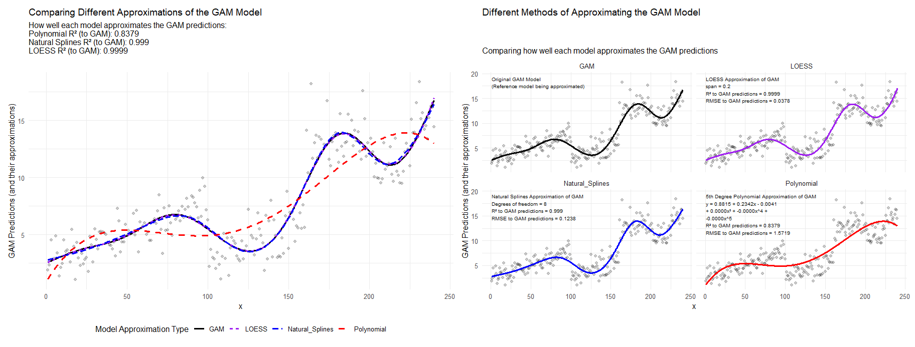
I have looked and looked on how this might be possible, and the only thing which makes sense to me is the following: After fitting the GAM model, predict multiple values of $y$ over a range of $x$ values , then fit a simpler model to these predicted values to approximate the GAM model (in a situation with multiple variables, you would hold all other variables at their mean value and just do this for one predictor and the response). This is my interpretation on how to do this in R:
# create grid for predictions
x_grid <- seq(min(data$x), max(data$x), length.out = 500)
gam_preds <- predict(gam_model, newdata = data.frame(x = x_grid))

# fit different models to GAM predictions

poly_model <- lm(gam_preds ~ poly(x_grid, degree = 5, raw = TRUE))
poly_preds <- predict(poly_model)

ns_model <- lm(gam_preds ~ ns(x_grid, df = 8))
ns_preds <- predict(ns_model)

loess_model <- loess(gam_preds ~ x_grid, span = 0.2)
loess_preds <- predict(loess_model)

calc_stats <- function(actual, predicted) {
    r2 <- round(cor(actual, predicted)^2, 4)
    rmse <- round(sqrt(mean((actual - predicted)^2)), 4)
    return(c(r2 = r2, rmse = rmse))
}

stats_poly <- calc_stats(gam_preds, poly_preds)
stats_ns <- calc_stats(gam_preds, ns_preds)
stats_loess <- calc_stats(gam_preds, loess_preds)

# Create equation for polynomial
coefs <- round(coef(poly_model), 4)
eq_terms <- character(length(coefs))
eq_terms[1] <- sprintf("%.4f", coefs[1])
for(i in 1:(length(coefs)-1)) {
    term <- sprintf("%.4fx%s", coefs[i+1],
                    if(i == 1) "" else if(i == 2) "²" else if(i == 3) "³" else paste0("^", i))
    eq_terms[i+1] <- if(coefs[i+1] >= 0) paste0(" + ", term) else paste0(" - ", abs(coefs[i+1]))
}
poly_eq <- paste0("y = ", paste(eq_terms, collapse = ""))

plot_data <- data.frame(
    x = x_grid,
    GAM = gam_preds,
    Polynomial = poly_preds,
    Natural_Splines = ns_preds,
    LOESS = loess_preds
)

plot_data_long <- tidyr::pivot_longer(plot_data,
                                      cols = -x,
                                      names_to = "Model",
                                      values_to = "y")

p1 <- ggplot() +
    geom_point(data = data, aes(x = x, y = y), alpha = 0.2) +
    geom_line(data = plot_data_long, aes(x = x, y = y, color = Model, linetype = Model),
              linewidth = 1) +
    scale_color_manual(values = c("GAM" = "black",
                                  "Polynomial" = "red",
                                  "Natural_Splines" = "blue",
                                  "LOESS" = "purple")) +
    theme_minimal() +
    labs(title = "All Models Comparison",
         subtitle = paste0("R² values:\n",
                           "Polynomial: ", stats_poly["r2"], "\n",
                           "Natural Splines: ", stats_ns["r2"], "\n",
                           "LOESS: ", stats_loess["r2"]),
         x = "x", y = "y") +
    theme(legend.position = "bottom")


labels <- list(
    GAM = paste0("Original GAM\n",
                 "Smoothing spline with default parameters"),
    Polynomial = paste0("Polynomial (degree 5)\n",
                        str_wrap(poly_eq, width = 30), "\n",
                        "R² = ", stats_poly["r2"], "\n",
                        "RMSE = ", stats_poly["rmse"]),
    Natural_Splines = paste0("Natural Splines\n",
                             "Degrees of freedom = 8\n",
                             "R² = ", stats_ns["r2"], "\n",
                             "RMSE = ", stats_ns["rmse"]),
    LOESS = paste0("LOESS\n",
                   "span = 0.2\n",
                   "R² = ", stats_loess["r2"], "\n",
                   "RMSE = ", stats_loess["rmse"])
)

p2 <- ggplot() +
    geom_point(data = data, aes(x = x, y = y), alpha = 0.2) +
    geom_line(data = plot_data_long, aes(x = x, y = y, color = Model),
              linewidth = 1) +
    facet_wrap(~Model, ncol = 2) +
    scale_color_manual(values = c("GAM" = "black",
                                  "Polynomial" = "red",
                                  "Natural_Splines" = "blue",
                                  "LOESS" = "purple")) +
    theme_minimal() +
    labs(title = "Individual Model Fits",
         x = "x", y = "y") +
    theme(legend.position = "none") +
    geom_text(data = data.frame(
        Model = names(labels),
        x = rep(min(data$x), length(labels)),
        y = rep(max(data$y) + 1, length(labels)),
        label = unlist(labels)
    ),
    aes(x = x, y = y, label = label),
    hjust = 0, vjust = 1, size = 2.5)

combined_plot <- p1 | p2
Thus, the natural question arises:
- Is this the correct methodology to obtain the model equation of the fitted GAM regression? (seems like we are introducing a new source of uncertainty/error proprogation)
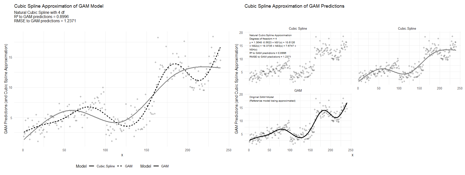
- If we can't get the final equation for the fitted GAM regression model, why not just fit a simpler regression model (e.g. cubic spline) on the original data that is able to directly provide the final fitted model equation?
x_grid <- seq(min(data$x), max(data$x), length.out = 500)
gam_preds <- predict(gam_model, newdata = data.frame(x = x_grid))

cubic_model <- lm(gam_preds ~ ns(x_grid, df = 4))  # using 4 degrees of freedom for simplicity
cubic_preds <- predict(cubic_model)

calc_stats <- function(actual, predicted) {
    r2 <- round(cor(actual, predicted)^2, 4)
    rmse <- round(sqrt(mean((actual - predicted)^2)), 4)
    return(c(r2 = r2, rmse = rmse))
}

stats_cubic <- calc_stats(gam_preds, cubic_preds)

basis_matrix <- ns(x_grid, df = 4)
coef_cubic <- coef(cubic_model)

eq_terms <- sprintf("%.4f", coef_cubic[1])  # intercept
for(i in 1:length(coef_cubic[-1])) {
    term <- sprintf("%.4f × NS%d(x)", coef_cubic[i+1], i)
    eq_terms <- paste(eq_terms, ifelse(coef_cubic[i+1] >= 0, "+", ""), term)
}
cubic_eq <- paste("y =", eq_terms)

plot_data <- data.frame(
    x = x_grid,
    GAM = gam_preds,
    `Cubic Spline` = cubic_preds
)

plot_data_long <- tidyr::pivot_longer(plot_data,
                                      cols = -x,
                                      names_to = "Model",
                                      values_to = "y")

p1 <- ggplot() +
    geom_point(data = data, aes(x = x, y = y), alpha = 0.2) +
    geom_line(data = plot_data_long, aes(x = x, y = y, color = Model, linetype = Model),
              linewidth = 1) +
    scale_color_manual(values = c("GAM" = "black", "Cubic Spline" = "red")) +
    theme_minimal() +
    labs(title = "Cubic Spline Approximation of GAM Model",
         subtitle = paste0("Natural Cubic Spline with 4 df\n",
                           "R² to GAM predictions = ", stats_cubic["r2"], "\n",
                           "RMSE to GAM predictions = ", stats_cubic["rmse"]),
         x = "x",
         y = "GAM Predictions (and Cubic Spline Approximation)",
         color = "Model",
         linetype = "Model") +
    theme(legend.position = "bottom")

labels <- list(
    GAM = "Original GAM Model\n(Reference model being approximated)",
    `Cubic Spline` = paste0("Natural Cubic Spline Approximation\n",
                            "Degrees of freedom = 4\n",
                            str_wrap(cubic_eq, width = 40), "\n",
                            "R² to GAM predictions = ", stats_cubic["r2"], "\n",
                            "RMSE to GAM predictions = ", stats_cubic["rmse"])
)

p2 <- ggplot() +
    geom_point(data = data, aes(x = x, y = y), alpha = 0.2) +
    geom_line(data = plot_data_long, aes(x = x, y = y, color = Model),
              linewidth = 1) +
    facet_wrap(~Model, ncol = 2) +
    scale_color_manual(values = c("GAM" = "black", "Cubic Spline" = "red")) +
    theme_minimal() +
    labs(title = "Cubic Spline Approximation of GAM Predictions",
         x = "x",
         y = "GAM Predictions (and Cubic Spline Approximation)") +
    theme(legend.position = "none") +
    geom_text(data = data.frame(
        Model = names(labels),
        x = rep(min(data$x), length(labels)),
        y = rep(max(data$y) + 1, length(labels)),
        label = unlist(labels)
    ),
    aes(x = x, y = y, label = label),
    hjust = 0, vjust = 1, size = 2.5)

combined_plot <- p1 | p2

print(combined_plot)
cat("\nCubic Spline Equation:\n", cubic_eq)


gam()are. $\endgroup$nsandpolywhich uses very parametric fits. If you think those are messy to deal with (I usually agree) then I would recommend using what I almost always use: restricted cubic splines (natural splines with truncated power basis). The Rrmspackage has alatexmethod that renders fitted equations in simplest form when using restricted cubic splines. $\endgroup$