5
$\begingroup$

I'm running a chi-square test on the distribution of a variable between different age groups. The data looks like this in R:

    a <- c(66,97, 48)
    b <- c(145,174,58)
    c <- c(129,128,58)
      
    M <- data.frame(cbind(a,b,c))
    colnames(M) <- c("18-34", "35-49","50-66")
    rownames(M) <- c("Below avg" , "Average","Above avg")
    view(M)

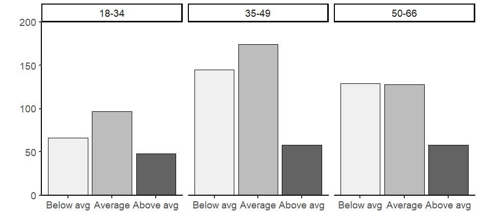
When plotted, the data from the youngest group appears similar in distribution to the middle one and different from the oldest one.

the plot

If I run an overall chi-square test, I get a non-significant difference:

X-squared = 8.6905, df = 4, p-value = 0.06932

However if I compare the age groups in pairs i get a significant difference between youngest and middle, and not between youngest and oldest.

data:  M[, 1:2]
X-squared = 6.0153, df = 2, p-value = 0.04941

data:  M3[, c(1, 3)]
X-squared = 5.2093, df = 2, p-value = 0.07393

I believe it has something to do with the unbalanced numbers of participants in each age group, even though the overall number of observations is rather large in each group. But I'm not sure if and how I should account for it.

$\endgroup$
6
  • 2
    $\begingroup$ Why are you using a threshold to say that the results are significant/not significant? 0.04941 is a degree of evidence against the null hypothesis rather similar to 0.06932 or 0.07393. $\endgroup$
    – J-J-J
    Commented Nov 29 at 9:46
  • 5
    $\begingroup$ I am reminded of Rosnow & Rosenthal: surely God loves $P=0.06$ nearly as much as $P=0.05$? $\endgroup$
    – PBulls
    Commented Nov 29 at 9:48
  • $\begingroup$ Your first paired comparison focuses on the largest difference only, therefore it has more statistical power than the omnibus test that takes into account all comparisons. $\endgroup$
    – Sointu
    Commented Nov 29 at 9:55
  • $\begingroup$ @J-J-J Sure, I understand your point. Still, I'm interested in why is the (slightly) larger difference between young-mid age and not young-old, which appear more different in the plot $\endgroup$
    – kinbeat
    Commented Nov 29 at 10:04
  • 6
    $\begingroup$ As an aside, grouping/discretization is not good practice. You implicitly treat a 35 year old as identical to a 49 year old, but both completely different than a 34 year old. I don't know about you, but I assure you that when I was 35, I felt much more like 34 than like 49. Similarly to whatever you group into "below average", "average" and "above average". Better to work with the original data, and look at correlations and scatterplots. Take a look at stats.stackexchange.com/q/68834/1352 $\endgroup$ Commented Nov 29 at 10:33

3 Answers 3

4
$\begingroup$

Actually, the $\chi^2$ test gives you exactly what it should, both for the omnibus test, and for the separate tests. The issue is with your interpretation of the graphs.

When you look at the 3 bar charts, they look quite the same; in fact, the heights of the bars seem very similar (e.g. the "above average" groups all have ~50 observations. But that "fools" your eyes. Compare instead the observed proportions; in the "young" group, the "above average" group is ~22.7% of the total. But in the "middle aged" group it is about 15.4%, about 1.5 times less; that difference in proportions, on such a large total number of counts, will be "significant". Now for the "old" group, that proportion is 18.4%; not quite as "significant". Overall, the young group is more different from the "middle aged" one than from the "old" one (even if, in both cases, it is quite different: after all, all your p-values are quite low).

$\endgroup$
0
7
$\begingroup$

Summarizing some of the comments and adding a bit:

  1. Don't compare p-values this way. In particular, don't interpret the difference between "significant" and "non-significant" this way. See Andrew Gelman's paper (title in case of link rot: The difference between 'significant' and 'not significant' is not, itself, statistically significant.

  2. The chi-square test statistic is not very intuitive but is very simple, arithmetically. You can look at the observed and expected for each cell and see what's happening.

  3. It would be better to use ungrouped data. But, if you haven't got that, it would be good to use a test that accounts for order, such as Jonckheere-Terpstra; an exact version is available in R in the DescTools package.

  4. You don't say what the "variable" is, but, if you are proposing that it varies by age, it might be better to use some form of regression, if that variable can be regarded as a dependent variable (or outcome, etc.)

$\endgroup$
2
  • $\begingroup$ Thank you for your answer. I understand why reasoning with p values in a dichotomic way is problematic, however that wasn't really the focus on my question, which was more on point 2 of your answer. I'll look into the test you suggested, basically i'm testing whether the outcome i'm measuring decreases faster in the subpopulation than what would be expected with age in the general population. $\endgroup$
    – kinbeat
    Commented Nov 29 at 13:27
  • 2
    $\begingroup$ The big picture here is elementary but fundamental: chi-square as an omnibus test statistic may seem to give contradictory results if associations are themselves in detail a little contradictory or complicated. I don't know whether to call that intuitive or not; it's a word I try to avoid. $\endgroup$
    – Nick Cox
    Commented Nov 29 at 14:45
4
$\begingroup$

The second and third groups are fairly similar, but have different numbers of observations.

More precisely there are about 20% more observations in the 35-49 group than in the 50-66 group. Extra data tends to tighten tests of proportions and can be enough to shift the test statistic across the $\chi^2$ critical value even before taking other issues into account.

To illustrate this, consider slightly adjusted data so the second and third group have the same proportions but different numbers:

aobs <- c(66, 97, 48)
cobs <- c(50, 125, 60)
bobs <- cobs * 1.2
print(bobs)
# 60 150  72

chisq.test(cbind(aobs, bobs))
# X-squared = 6.365, df = 2, p-value = 0.04148

chisq.test(cbind(aobs, cobs))
# X-squared = 5.7971, df = 2, p-value = 0.0551

Looking at all three groups increases the test statistic further, but it also increases the number of degrees of freedom, so instead of a $\chi^2_2$ test you are now comparing to a $\chi^2_4$ critical value, meaning the critical value has grown by more; the overall result appears less significant (a higher $p$-value) than the subtests largely because the proportions in the second and third group are so close to each other in this artificial data.

chisq.test(cbind(aobs, bobs, cobs))
# X-squared = 8.1999, df = 4, p-value = 0.08452

If instead you had combined the second and third groups, you would get the same test statistic but greater significance.

chisq.test(cbind(aobs, bobs + cobs))
# X-squared = 8.1999, df = 2, p-value = 0.01657

All this post-hoc rationalisation probably does not help the quality of conclusions, which is why you should decide the tests you are going to perform before you see the data.

$\endgroup$

Your Answer

By clicking “Post Your Answer”, you agree to our terms of service and acknowledge you have read our privacy policy.

Not the answer you're looking for? Browse other questions tagged or ask your own question.