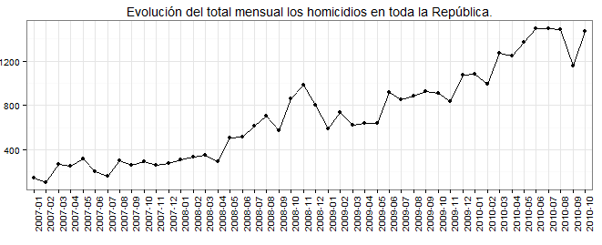
A dynamic panel model might make sense if you have a eye-for-an-eye retaliation model for homicides. For example, if the homicide rate was largely driven by gangs feuds, the murders at time $t$ might well be a function of the deaths at $t-1$, or other lags.
I am going to answer your questions out of order. Suppose the DGP is
\begin{equation}
y_{it}=\delta y_{it-1}+x_{it}^{\prime}\beta+\mu_{i}+v_{it},
\end{equation}
where the errors $\mu$ and $v$ are independent of each other and among themselves. You're interested in conducting the test of whether $\delta = 0$ (question 2).
If you use OLS, it's easy to see that $y_{it-1}$ and the first part of the error are correlated, which renders OLS biased and inconsistent, even when there's no serial correlation in $v$. We need something more complicated to do the test.
The next thing you might try is the fixed effects estimator with the within transformation, where you transform the data by subtracting each unit's average $y$, $\bar y_{i}$, from each observation. This wipes out $\mu$, but this estimator suffers from Nickell bias, which bias does not go away as the number of observations $N$ grows, so it is inconsistent for large $N$ and small $T$ panels. However, as $T$ grows, you get consistency of $\delta$ and $\beta$. Judson and Owen (1999) do some simulations with $N=20,100$ and $T=5,10,20,30$ and found the bias to be increasing in $\delta$ and decreasing in $T$. However, even for $T=30$, the bias could be as much as $20\%$ of the true coefficient value. That's bad news bears! So depending on the dimensions of you panel, you may want to avoid the within FE estimator. If $\delta > 0$, the bias is negative, so the persistence of $y$ is underestimated. If the regressors are correlated with the lag, the $\beta$ will also be biased.
Another simple FE approach is to first-difference the data to remove the fixed effect, and use $y_{it-2}$ to instrument for $\Delta y_{it-1} = y_{it-1}-y_{it-2}$. You also use $x_{it}-x_{it-1}$ as an instrument for itself. Anderson and Hsiao (1981) is the canonical reference. This estimator is consistent (as long as the explanatory $X$s are pre-determined and the original error terms are not serially correlated), but not fully efficient since it does not use all the available moment conditions and does not use the fact that the error term is now differenced. This would probably be my first choice. If you think that $v$ follow an AR(1) process, can use third and fourth lags of $y$ instead.
Arellano and Bond (1991) derive a more efficient generalized method of moments (GMM) estimator, which has been extended since, relaxing some of the assumptions. Chapter 8 of Baltagi's panel book is a good survey of this literature, though it does not deal with lag selection as far as I can tell. This is state of the art 'metrics, but more technically demanding.
I think the plm package in R has some of these built in. Dynamic panel models have been in Stata since version 10, and SAS has the GMM version at least. None of these are count data models, but that may not be a big deal depending on your data. However, here's one example of a GMM dynamic Poisson panel model in Stata.
The answer to your first question is more speculative. If you leave out the lagged $y$ and first difference, I believe that $\beta$ can still be estimated consistently, though less precisely since the variance is now larger. If that is the parameter you care about, that may be acceptable. What you loose is that you cannot say whether there were a lot of homicides in area X because they were lots last month or because area X has a propensity for violence. You give up the ability to distinguish between state dependence and unobserved heterogeneity (question 1).

