The positive stable distribution in R

Question

Positive stable distributions are described by four parameters: the skewness parameter $\beta\in[-1,1]$, the scale parameter $\sigma>0$, the location parameter $\mu\in(-\infty,\infty)$, and the so-called index parameter $\alpha\in(0,2]$. When $\beta$ is zero the distribution is symmetric around $\mu$, when it is positive (resp. negative) the distribution is skewed to the right (resp. to the left). Stable distributions allow fat tails when $\alpha$ decreases.

When $\alpha$ is strictly less than one and $\beta=1$ the support of the distribution restricts to $(\mu,\infty)$.

The density function only has a closed-form expression for some particular combinations of values for the parameters. When $\mu=0$, $\alpha<1$, $\beta=1$, and $\sigma=\alpha$ it is (see formula (4.4) here):

$f(y) = -\frac{1}{\pi y} \sum_{k=1}^{\infty} \frac{\Gamma(k\alpha+1)}{k!} (-y^{-\alpha})^k \sin(\alpha k \pi)$

It has infinite mean and variance.

Question

I would like to use that density in R. I use

> alpha <- ...
> dstable(y, alpha=alpha, beta=1, gamma=alpha, delta=0, pm=1)

where the dstable function comes with the fBasics package.

Can you confirm this is the right way to compute that density in R?

Thank you in advance!

EDIT

One reason why I am suspicious is that, in the output, the value of delta is different from that in the input. Example:

> library(fBasics)
> alpha <- 0.4
> dstable(4, alpha=alpha, beta=1, gamma=alpha, delta=0, pm=1)
[1] 0.02700602
attr(,"control")
   dist alpha beta gamma    delta pm
stable   0.4    1   0.4 0.290617  1

Answer 1

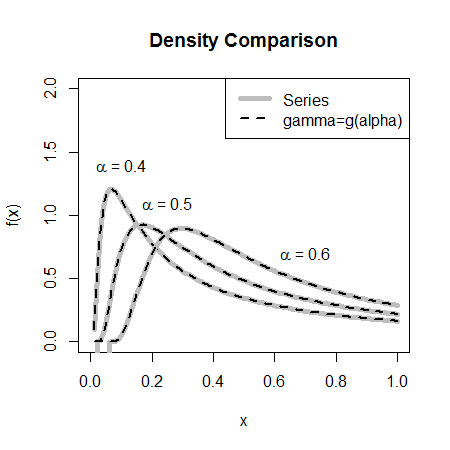
The short answer is that your $\delta$ is fine, but your $\gamma$ is wrong. In order to get the positive stable distribution given by your formula in R, you need to set $$ \gamma = |1 - i \tan \left(\pi \alpha / 2\right)|^{-1/\alpha}. $$

The earliest example I could find of the formula you gave was in (Feller, 1971), but I've only found that book in physical form. However (Hougaard, 1986) gives the same formula, along with the Laplace transform $$ \mathrm{L}(s) = \mathrm{E}\left[\exp(-sX)\right] = \exp\left(-s^\alpha\right). $$ From the stabledist manual (stabledist is used in fBasics), the pm=1 parameterization is from (Samorodnitsky and Taqqu, 1994), another resource whose online reproduction has eluded me. However (Weron, 2001) gives the characteristic function in Samorodnitsky and Taqqu's parameterization for $\alpha \neq 1$ to be $$ \varphi(t) = \mathrm{E}\left[\exp(i t X) \right] = \exp\left[i \delta t - \gamma^\alpha |t|^\alpha \left(1 - i \beta \mathrm{sign}(t) \tan{\frac{\pi \alpha}{2}} \right) \right]. $$ I've renamed some parameters from Weron's paper to coinside with the notation we're using. He uses $\mu$ for $\delta$ and $\sigma$ for $\gamma$. In any case, plugging in $\beta=1$ and $\delta=0$, we get $$ \varphi(t) = \exp\left[-\gamma^\alpha |t|^\alpha \left(1 - i \mathrm{sign}(t) \tan \frac{\pi \alpha}{2} \right) \right]. $$

Note that $(1 - i \tan (\pi \alpha / 2)) / |1 - i \tan(\pi \alpha / 2)| = \exp(-i \pi \alpha / 2)$ for $\alpha \in (0, 1)$ and that $i^\alpha = \exp(i \pi \alpha / 2)$. Formally, $\mathrm{L}(s)=\varphi(is)$, so by setting $\gamma = |1 - i \tan \left(\pi \alpha / 2\right)|^{-1/\alpha}$ in $\varphi(t)$ we get $$ \varphi(is) = \exp\left(-s^\alpha\right) = \mathrm{L}(s). $$ One interesting point to note is that the $\gamma$ that corresponds to $\alpha=1/2$ is also $1/2$, so if you were to try $\gamma=\alpha$ or $\gamma=1-\alpha$, which is actually not a bad approximation, you end up exactly correct for $\alpha=1/2$.

Here's an example in R to check correctness:

library(stabledist)

# Series representation of the density
PSf <- function(x, alpha, K) {
  k <- 1:K
  return(
    -1 / (pi * x) * sum(
      gamma(k * alpha + 1) / factorial(k) * 
        (-x ^ (-alpha)) ^ k * sin(alpha * k * pi)
    )
  )
}

# Derived expression for gamma
g <- function(a) {
  iu <- complex(real=0, imaginary=1)
  return(abs(1 - iu * tan(pi * a / 2)) ^ (-1 / a))
}

x=(1:100)/100
plot(0, xlim=c(0, 1), ylim=c(0, 2), pch='', 
     xlab='x', ylab='f(x)', main="Density Comparison")
legend('topright', legend=c('Series', 'gamma=g(alpha)'),
       lty=c(1, 2), col=c('gray', 'black'),
       lwd=c(5, 2))
text(x=c(0.1, 0.25, 0.7), y=c(1.4, 1.1, 0.7), 
     labels=c(expression(paste(alpha, " = 0.4")),
              expression(paste(alpha, " = 0.5")),
              expression(paste(alpha, " = 0.6"))))

for(a in seq(0.4, 0.6, by=0.1)) {
  y <- vapply(x, PSf, FUN.VALUE=1, alpha=a, K=100)
  lines(x, y, col="gray", lwd=5, lty=1)
  lines(x, dstable(x, alpha=a, beta=1, gamma=g(a), delta=0, pm=1), 
        col="black", lwd=2, lty=2)
}

$\hskip1in$

1. Feller, W. (1971). An Introduction to Probability Theory and Its Applications, 2, 2nd ed. New York: Wiley.
2. Hougaard, P. (1986). Survival Models for Heterogeneous Populations Derived from Stable Distributions, Biometrika 73, 387-396.
3. Samorodnitsky, G., Taqqu, M.S. (1994). Stable Non-Gaussian Random Processes, Chapman & Hall, New York, 1994.
4. Weron, R. (2001). Levy-stable distributions revisited: tail index > 2 does not exclude the Levy-stable regime, International Journal of Modern Physics C, 2001, 12(2), 209-223.

Answer 2

What I think is happening is that in the output delta may be reporting an internal location value, while in the input delta is describing the shift. [There seems to be a similar issue with gamma when pm=2.] So if you try increasing the shift to 2

> dstable(4, alpha=0.4, beta=1, gamma=0.4, delta=2, pm=1)
[1] 0.06569375
attr(,"control")
   dist alpha beta gamma    delta pm
 stable   0.4    1   0.4 2.290617  1

then you add 2 to the location value.

With beta=1 and pm=1 you have a positive random variable with a distribution lower bound at 0.

> min(rstable(100000, alpha=0.4, beta=1, gamma=0.4, delta=0, pm=1))
[1] 0.002666507

Shift by 2 and the lower bound rises by the same amount

> min(rstable(100000, alpha=0.4, beta=1, gamma=0.4, delta=2, pm=1))
[1] 2.003286

But if you want the delta input to be the internal location value rather than the shift or lower bound, then you need to use a different specification for the parameters. For example if you try the following (with pm=3 and trying delta=0 and the delta=0.290617 you found earlier), you seem to get the same delta in and out. With pm=3 and delta=0.290617 you get the same density of 0.02700602 you found earlier and a lower bound at 0. With pm=3 and delta=0 you get a negative lower bound (in fact -0.290617).

> dstable(4, alpha=0.4, beta=1, gamma=0.4, delta=0, pm=3)
[1] 0.02464434
attr(,"control")
   dist alpha beta gamma delta pm
 stable   0.4    1   0.4     0  3
> dstable(4, alpha=0.4, beta=1, gamma=0.4, delta=0.290617, pm=3)
[1] 0.02700602
attr(,"control")
   dist alpha beta gamma    delta pm
 stable   0.4    1   0.4 0.290617  3
> min(rstable(100000, alpha=0.4, beta=1, gamma=0.4, delta=0, pm=3))
[1] -0.2876658
> min(rstable(100000, alpha=0.4, beta=1, gamma=0.4, delta=0.290617, pm=3))
[1] 0.004303485

You may find it easier simply to ignore delta in the output, and so long as you keep beta=1 then using pm=1 means delta in the input is the distribution lower bound, which it seems you want to be 0.

Answer 3

Also of note: Martin Maechler just refactored the code for the stable distributed and added some improvements.

His new package stabledist will be used by fBasics as well, so you may want to give this a look as well.