9
$\begingroup$

I have two different measuring instruments, A and B, both measure the same physical property $x$ of an object but with different "quality": B gives measurements with a known uncertainty while I do not know the uncertainty in the measurements given by A.

I have $N$ distinct objects and I measure the property $x$ for all of them with A, so I get a list of measurements $L_A=\{x_{A1}, x_{A2},\ldots,x_{AN}\}$ where $x_{Ai}$ is the measurement of the property $x$ for the $i$-th object.

The objects are not labeled so, given an object, I just know that its measurement belongs to $L_A$ but I am not able to extract the measurement from $L_A$. Furthermore, I cannot use A to measure an object that I have already measured in the past with A.

Then I randomly choose $M \lt N$ objects from the $N$ objects. I measure all the $M$ objects of the sample with B and I get a list of measurements $L_B=\{x_{B1}, x_{B2},\ldots,x_{BM}\}$. Please note that the index in the subscript is not a label for the object so I cannot directly compare $x_{A1}$ with $x_{B1}$.

Is it possible to estimate the uncertainty in the measurements given by A with the above data?

I was thinking about comparing the empirical cumulative distribution function of $L_A$ with the one of $L_B$ but it is just an idea and I am not able to elaborate it further.

Is there any established standards which cover my problem? For example I found references to "ISO 5725: Accuracy (trueness and precision) of measurement methods and results" but I have not access to it.

Update:

I found my question similar to How to test if reading from two devices are significantly different? where I read the answer by Michael Lew, he suggests the paper LUDBROOK, John. Statistical techniques for comparing measurers and methods of measurement: a critical review. Clinical and Experimental Pharmacology and Physiology, 2002, 29.7: 527-536. but unfortunately it seems to me that the paper requires the pairing between the measurements.

Update 2:

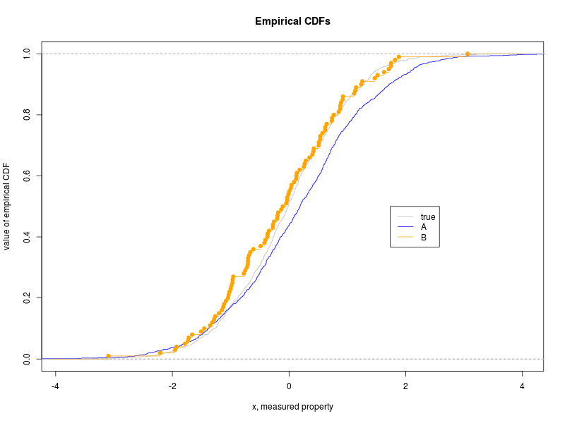
I have written an R script to simulate my problem.

set.seed(42)

instrument_measurement <- function(true_value,gain,offset,dispersion)
# The instrument has three parameters: the true_value is transformed by means
# of a linear transformation described by parameters offset and gain; then there
# is a dispersion parameter. An ideal instrument would have gain=1, offset=0
# and dispersion that approaches to zero.
{
  return(rnorm(length(true_value),mean=gain*true_value-offset,sd=dispersion))
}

N=1000
true_mean = 0
true_sd = 1
# I simulate the property to be measured for N objects, here the property is
# normally distributed...
true_values = rnorm(N,mean=true_mean,sd=true_sd)

# but it could also be a mixture of normal distributions:

# components <- sample(1:3,prob=c(1/7,5/7,1/7),size=N,replace=TRUE)
# mus <- c(-0.2,0,+0.3)
# sds <- sqrt(c(0.05,0.05,0.05))
# true_values <- rnorm(n=N,mean=mus[components],sd=sds[components])
# plot(density(true_values))


# The "quality" of instrument B is "good enough" to measure the true values:
gain_B = 1
offset_B = true_sd/10
dispersion_B = true_sd/10

# The instrument B has a lower "quality" than the one of instrument A:
gain_A = 1.1*gain_B
offset_A=-2*offset_B
dispersion_A=5*dispersion_B

# I simulate the measuremente made by instrument A:
L_A = instrument_measurement(true_values,gain_A,offset_A,dispersion_A)

# I make the sample:
sample_to_measure_with_B = sample(true_values,100,replace=F)

# I simulate the measuremente made by instrument B:
L_B = instrument_measurement(sample_to_measure_with_B,gain_B,offset_B,dispersion_B)

# I plot the empirical CDF of the true values, of the measurements made with
# instrument A and of the measurements made with instrument B
plot(ecdf(true_values),col="grey",main="",xlab="x, measured property",ylab="value of empirical CDF")
lines(ecdf(L_A),col="blue")
lines(ecdf(L_B),col="orange")
legend(x=(max(true_values)+mean(true_values))/2,y=.5,legend=c("true","A","B"),col=c("grey","blue","orange"),lty=c(1,1,1))
title("Empirical CDFs")

Referring to the script, is is possible to estimate gain_A, offset_A and dispersion_A from L_A and L_B? What would be the uncertainties in the estimates?

I had an inelegant idea of defining a cost function and try to minimize it in the space of the parameters gain, offset and dispersion:

function <- ecdf_distance(ecdf1,ecdf2)
{
# return 0 if ecdf1 is "equal" to ecdf2
# return a positive scalar that measures the difference between ecdf1 and ecdf2
}

function <- cost(parameters)
{
L = instrument_measurement(L_B,parameters$gain,parameter$offset,parameter$dispersion)
return(ecdf_distance(ecdf(L_A),ecdf(L))
}

I made some test keeping gain=1 but with no luck... the cost function seems constant with respect to dispersion... I am afraid I lack some theory/math about the problem :-)
enter image description here

$\endgroup$
2
  • $\begingroup$ Are these $N$ objects supposed to be similar (same dimensions)? $\endgroup$
    – Baumann
    Commented Feb 17, 2014 at 20:58
  • $\begingroup$ @Baumann Yes they are. The $N$ objects are supposed to be similar. $\endgroup$ Commented Feb 18, 2014 at 17:41

2 Answers 2

3
+50
$\begingroup$

The model you use to "simulate your problem" can be used almost verbatim to estimate the parameters you are interested in using Bayesian estimation. Here is the model I'll use (using the same notation as you):

$$ L_B \sim \mathrm{Normal}(\mu, \sigma) \\ x_i \sim \mathrm{Normal}(\mu, \sigma) \mathrm{\ for\ i\ from\ 1\ to\ N} \\ L_{Ai} \sim \mathrm{Normal}(x_i \cdot \mathrm{gain} - \mathrm{offset}, \mathrm{dispersion}) \mathrm{\ for\ i\ from\ 1\ to\ N} \\ $$

The glaring omision in this model compared to your problem is that I don't include the assumption that some of the same $x_i$s that got measured by B could then be measured again by A. This could probably be added, but I'm not completely sure how.

This model is implemented in R & JAGS below using very vague, almost flat priors, the data used is the one you generated in your question:

library(rjags)

model_string <- "model{
  for(i in 1:length(L_B)) {
  L_B[i] ~ dnorm(mu, inv_sigma2) # <- reparameterizing sigma into precision 
                                 #    needed because of JAGS/BUGS legacy.  
  }
  for(i in 1:length(L_A)) {
    x[i] ~ dnorm(mu, inv_sigma2)
    L_A[i] ~ dnorm(gain * x[i] - offset , inv_dispersion2)
  }

  mu ~ dnorm(0, 0.00001)
  inv_sigma2 ~ dgamma(0.0001, 0.0001) 
  sigma <- sqrt(1 / inv_sigma2)
  gain ~ dnorm(0, 0.00001) T(0,)
  offset ~ dnorm(0, 0.00001)
  inv_dispersion2 ~ dgamma(0.0001, 0.0001)
  dispersion <- sqrt(1 / inv_dispersion2)
}"

Let's run it and see how well it does:

model <- jags.model(textConnection(model_string), list(L_A = L_A, L_B = L_B), n.chains=3)
update(model, 3000)
mcmc_samples <- coda.samples(model, c("mu", "sigma", "gain", "offset", "dispersion"), 200000, thin=100)
apply(as.matrix(mcmc_samples), 2, quantile, c(0.025, 0.5, 0.975))
##       dispersion   gain      mu   offset  sigma
## 2.5%     0.01057 0.1366 -0.3116 -0.51836 0.9365
## 50%      0.18657 1.0745 -0.1099 -0.26950 1.0675
## 97.5%    1.20153 1.2846  0.1051 -0.04409 1.2433

The resulting estimates are reasonably close to the values you used when you generated the data:

c(gain_A, offset_A, dispersion_A)
## [1]  1.1 -0.2  0.5

...except for, perhaps, dispersion. But with more data, perhaps more informed priors and running the MCMC sampling longer this estimate should be better.

$\endgroup$
7
  • $\begingroup$ @uvts_cvs Please tell me if you want me to clarify something! $\endgroup$ Commented Feb 24, 2014 at 11:09
  • $\begingroup$ +1, thank you very much for your answer. You wrote about the "glaring omission": let's say we find a way to include the information that some objects measured by A is then also measured by B, do you think that then the estimates will be better? $\endgroup$ Commented Feb 24, 2014 at 18:28
  • $\begingroup$ Could you suggest me any practical introduction to the Bayesian Estimation (BE)? My ideal reference would be a clear explanation of the theory of the BE (I am not scared of calculus) with examples in R (BUGS, JAGS, Stan); I am not interested a lot in the details of the various algorithms used in BE. When I say that I am not scared of calculus I mean that I love explanations like the one in HOGG, David W. Data analysis recipes: Probability calculus for inference. arXiv preprint arXiv:1205.4446, 2012. What really scares me: johndcook.com/blog/2008/02/23/everything-begins-with-p $\endgroup$ Commented Feb 24, 2014 at 19:34
  • $\begingroup$ Ok, a really great book is Doing Bayesian Data Analysis another book that's really hands on is the Bugs book. I don't know of any good web resource (but would love to know about) $\endgroup$ Commented Feb 24, 2014 at 22:09
  • $\begingroup$ Regarding the "glaring omission". For the dataset you have generated I don't think it matters that much (except it would be nice to solve the problem properly). For a much much smaller dataset it could matter more. $\endgroup$ Commented Feb 24, 2014 at 22:12
4
$\begingroup$

I'm more of an engineering guy, not a stats guy, so lets talk nuts-and-bolts.

Find:

  • estimated object metric uncertainty (state covariance)
  • (possibly) an established standard measurement for finding measurment uncertainty.

Given:

  • random replacement of the object measured after each measurement, so paired comparison is not allowed.
  • two measurement tools with different measurement uncertainty, one of whose uncertainty is not characterized.

Considerations:

  • Calibration. Most measurement systems are calibrated against high quality standards and so they have minimal bias. I should be able to assume this, but your system indicates bias as an issue.
  • Sample size. Taking 100 measurements is pretty weak. I prefer at least 300, but that is related to my data. You need to make sure that you get enough samples to minimize the error in your estimates, but not so much that you are buried. I can easily get 10M samples, but it is beyond the scope of MatLab and my laptop to do anything more than basics with that many rows.

Approach:

  • convert your code from R to a language I know well, MatLab.
  • look at CDF-domain interploation and scatterplots.

MatLab of your code:

function MySimulation

%houekeeping
clc;

%parameters
N=1000
true_mean = 0
true_sd = 1
% I simulate the property to be measured for N objects, here the property is
% normally distributed...
true_values = normrnd(true_mean,true_sd,N,1);

% but it could also be a mixture of normal distributions:
% it could be anything.  A Gaussian mixture is crazy-tame compared to what
% it could be, but we have to assume something to start this.

% The "quality" of instrument B is "good enough" to measure the true values:
gain_B = 1;
offset_B = true_sd/10;
dispersion_B = true_sd/10;

% The instrument B has a lower "quality" than the one of instrument A:
gain_A = 1.1*gain_B;
offset_A=-2*offset_B;
dispersion_A=5*dispersion_B;

% I simulate the measuremente made by instrument A:
L_A = instrument_measurement(true_values,gain_A,offset_A,dispersion_A);

% I make the sample:
% sample_to_measure_with_B = sample(true_values,100,replace=F)
sample_to_measure_with_B = randsample(true_values,100);

% I simulate the measuremente made by instrument B:
L_B = instrument_measurement(sample_to_measure_with_B,gain_B,offset_B,dispersion_B);

% I plot the empirical CDF of the true values, of the measurements made with
% instrument A and of the measurements made with instrument B

figure(1); clf; hold on
h1=cdfplot(true_values);
set(h1,'Color',0.5.*[1,1,1],'Linewidth',2);

h2=cdfplot(L_A);
set(h2,'Color','b','Marker','+');

h3=cdfplot(L_B);
set(h3,'Color',[1,0.65,0],'Marker','o');

legend('true','A','B','location','northwest')
title('Empirical CDFs')
xlabel('x-measured property')
ylabel('value of empirical CDF')


function [out] = instrument_measurement(true_value,gain,offset,dispersion)
% The instrument has three parameters: the true_value is transformed by means
% of a linear transformation described by parameters offset and gain; then there
% is a dispersion parameter. An ideal instrument would have gain=1, offset=0
% and dispersion that approaches to zero.
out=normrnd(gain*true_value-offset,dispersion,length(true_value),1);
return

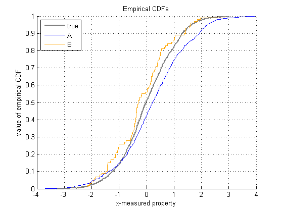
Your picture, translated: enter image description here

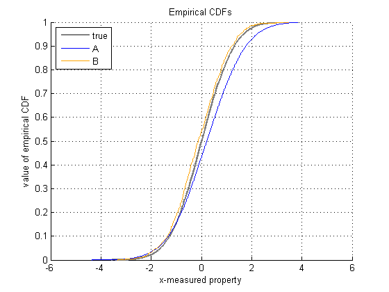
10x Higher sampling: enter image description here

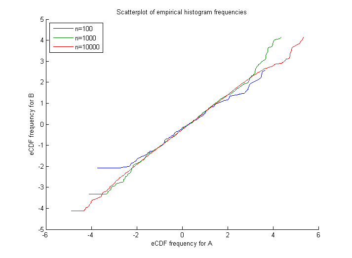
Now when we plot the A vs. B using the following

[xa,fa]=ecdf(L_A);
[xb,fb]=ecdf(L_B);

xb2=xa;
fb2=interp1(xb,fb,xb2);

we get the this:

enter image description here

If you look at it, you see that, except for runaway at the tails, the relationship between these two distributions is essentially linear. It is scale and offset. I would use sample size to figure out where to truncate the tails, then fit an analytic line through that. Then I can translate from one sensor reading to another.

The trick of mapping through CDF's is how to deal with many distributions. You need to make sure that your sample size is high enough to capture the characteristics of the underlying distribution.

If you were dealing with one bite at a time, iteratively instead of 10k samples at a time, then you could use a kalman filter to determine the mean and variance, or the transform between A and B. The preceding is a "rev1" brute force sort of approach. It is inelegant. It has holes and weaknesses. It is not strongly characterized. It does not stand on amazingly strong theoretical foundations. It is, however, reasonably quick and "good enough" which are also nice measures of goodness.

About Welch has a great introduction. (link)

A keyword for this is "sensor fusion". Here is a second link on the topic. (link)

Best of luck.

$\endgroup$
3
  • $\begingroup$ I am sorry but I do not grasp how I can apply the Kalman Filter to my problem. Could you please elaborate a bit further? Thank you. $\endgroup$ Commented Feb 20, 2014 at 17:20
  • $\begingroup$ +1. Based on your scatterplot you wrote that you can estimate scale (which I called gain) and offset but I have a third parameter called dispersion that is not accounted for... $\endgroup$ Commented Feb 24, 2014 at 18:21
  • 1
    $\begingroup$ The gaussian distribution is a 2-parameter distribution. It only has mean and variance (aka standard deviation). offset is about bias/accuracy and scale is about variation/precision. I will think a bit, and see if I can make a "fminsearch" or such that can do the fitting of your second piece of code. No promises on timing. $\endgroup$ Commented Feb 24, 2014 at 19:25

Your Answer

By clicking “Post Your Answer”, you agree to our terms of service and acknowledge you have read our privacy policy.

Not the answer you're looking for? Browse other questions tagged or ask your own question.