4
$\begingroup$

I`d like to extract the parameters of a two-component mixture distribution of noncentral student t distributions which first has to be fitted to a one-dimensional sample.

My question is closely related to this thread, but as pointed out I want to use Student t components for the mixture: Which R package to use to calculate component parameters for a mixture model

There are many packages for R that are capable of handling mixture distributions in one way or another. Some in the context of a Bayesian framework requiring kernels. Some in a regression framework. Some in a nonparametric framework. ...

In general the "mixdist"-package seems to come closest to my wish. This package fits parametric mixture distributions to a sample of data. Unfortunately it doesn`t support the student t distribution.

I have also tried to manually set up a likelihood function as described here: https://stackoverflow.com/questions/6485597/r-how-to-fit-a-large-dataset-with-a-combination-of-distributions But my result is far from perfect.

The "gamlss.mx"-package might be helping, but originally it seems to be set up for another context, i.e. regression. I tried to regress my data on a constant and then extract the parameters for the estimated mixture error distribution. Is this a valid approach?

But with this approach the estimated parameters seem to be not directly accessable individually by some command (such as fit1$sigma). And more importantly there seem to be serious estimation problems even in pretty simple and nonambiguous cases. E.g. in example 2 (see syntax below) I simulated a mixture which looks like this:
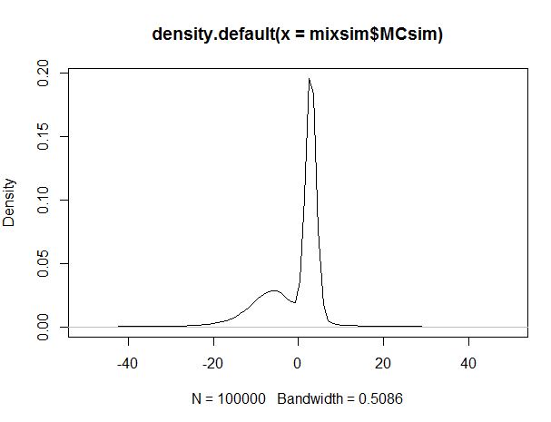
kernel density estimate of the mixture

When trying to fit a two-component student t mixture to these data either I get this error message (the deeper meaning of which I don't understand):

enter image description here

or I get wrong results (convergenve is reached only after approximately two hours as can be seen from the output):
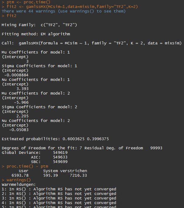
enter image description here

The means could be estimated well, but both the variance and the degrees of freedom are estimated badly. In the TF2 implementation of the student t, the sigma parameter denotes the standard deviation. Its estimate is NEGATIVE for the first component! And for the second component the degrees of freedom estimate is also NEGATIVE. Probably one should not use these results in practice :(

By the way: Is there a way to restrict these degree-of-freedom coefficient estimates to be natural numbers?

The following syntax is my gamlss.mx-setup so far:

library(gamlss.dist)
library(gamlss.mx)
library(MASS)

# example 1 (real data):
data(geyser)
plot(density(geyser$waiting) )
fit1 <- gamlssMX( waiting~1,data=geyser,family="TF2",K=2 )
fit1
# works fine

# example 2 (simulated data):
N <- 100000
components <- sample(1:2,prob=c(0.6,0.4),size=N,replace=TRUE)
mus <- c(3,-6)    # denotes the mean of component 1 and 2, respectively
sds <- c(1,9)     # ... the standard deviations
nus <- c(25,3)    # ... the degrees of freedom
mixsim <-data.frame(rTF2( N,mu=mus[components],sigma=sds[components],nu=nus[components] ))
colnames(mixsim) <- "MCsim"
plot(density(mixsim$MCsim) , xlim=c(-50,50))
fit2 <- gamlssMX(MCsim~1,data=mixsim,family="TF2",K=2)
fit2
# error message or strange results (this also happens when using a sample of S&P500 returns)

I would be very grateful for any advice! I've read through many related manuals and vignettes so far but I`m still lost.

Thanks a lot in advance!! Jo

$\endgroup$
8
  • $\begingroup$ I am somewhat curious why you would choose non-central Student-t components, because they are not very computationally tractable: they have only a limited number of moments of small order and most of their properties are difficult to compute. What theory of the genesis of your data leads to such a mixture model? $\endgroup$
    – whuber
    Commented May 1, 2014 at 22:42
  • $\begingroup$ I want to use the non-central student t components because I aim at a scenario analysis framework to test the performance of dynamically modeled risk measures such as Value at Risk or Expected Shortfall for a project at uni. A dynamically adjusted mixture distribution of two such components can generally reflect the characteristics of returns. Moreover, the two components can be nicely interpreted as two scenarios (quiet market versus stress period) and therefore subjectively chosen or manipulated. But to fit them to historical data I need some estimation technique for their parameters. $\endgroup$
    – Joz
    Commented May 2, 2014 at 7:37
  • $\begingroup$ What I am asking is why: Why should a noncentral t distribution be a good choice to model "returns" (presumably for some investment prospect)? There are potentially many other more tractable families of qualitatively similar distributions that can do the same thing. What is it about these investments that suggests using noncentral t distributions to the exclusion of all else? $\endgroup$
    – whuber
    Commented May 2, 2014 at 14:51
  • $\begingroup$ A gaussian mixture would be too unflexible (I don't want to work with more than 2 components at a time due to intuition issues in setting up scenarios). Other distributions easily get even more complicated I think (e.g. skewed distributions). One very important aspect for me is that there should be (implicit) analytical formulas for the Value at Risk and the Expected Shortfall (which I have set up for the t mixture already). So this gives nice opportunities for performance testing of risk measures. But feel free to suggest another alternative. I'm open minded! $\endgroup$
    – Joz
    Commented May 2, 2014 at 15:38
  • $\begingroup$ It depends on which aspects of risk are important for you to capture. Now that I know you are assessing risk, I appreciate the value of using components that might have infinite moments. $\endgroup$
    – whuber
    Commented May 2, 2014 at 16:28

2 Answers 2

1
$\begingroup$

Since I'm quite interested in the mixture analysis, I took the liberty to perform a brief research to see, if there is something new (both due to my limited knowledge of the subject and due to time elapsed since the original posting) on the topic, related to your question. The results follow.

In terms of the reasons of why one would want to use Student-t distribution instead of Gaussian (based on the discussion in comments) in the context of financial industry, I have found this interesting presentation slides document, which clarified the rationale to me (starting from page 4).

In terms of the algorithms for Student-t distribution's mixture analysis, I have discovered several interesting research papers, such as this general paper and this financial industry-focused paper.

Finally, in terms of the R packages that are focused on or support Student-t distribution-based mixture analysis, I have discovered several packages that are either relatively new or simply haven't been mentioned in previous discussion. So, I thought it might be beneficial to list them:

$\endgroup$
0
$\begingroup$

I am still curious if there a way to restrict the degree-of-freedom coefficient estimates to be natural numbers. But I think the rest is solved:

library(gamlss.dist)
library(gamlss.mx)

N <- 5000
components <- sample(1:2,prob=c(0.6,0.4),size=N,replace=TRUE)
mus <- c(3,-6)
sds <- c(1,9)
nus <- c(25,5)
mixsim <- data.frame(rTF2(N,mu=mus[components],sigma=sds[components],nu=nus[components]))
colnames(mixsim) <- "MCsim"
plot(density(mixsim$MCsim) , xlim=c(-50,50))

fit <- gamlssMX(MCsim~1,data=mixsim,family="TF2",K=2
     , control = MX.control( cc = 1e-04, n.cyc = 200, trace = T, seed = 2453385 , plot = T ) )

mu1 = as.numeric( coef(fit$models[[1]], "mu") ); mu1
    sd1 = exp( as.numeric( coef(fit$models[[1]], "sigma") ) ); sd1
nu1 = exp( as.numeric( coef(fit$models[[1]], "nu") ) ); nu1
    mu2 = as.numeric( coef(fit$models[[2]], "mu") ); mu2
sd2 = exp( as.numeric( coef(fit$models[[2]], "sigma") ) ); sd2
    nu2 = exp( as.numeric( coef(fit$models[[2]], "nu") ) ); nu2

First of all the sigma and nu parameter are fitted on a log-scale. This accounts for the negative estimates before. After transforming them back results are meaningful.

Secondly there seems to be no direct extractor-functions for the parameter estimates. But digging into the code revealed the solution given above.

Thirdly estimation is slow. Fitting a Student's t mixture to 100000 observations takes ages. So after reducing the sample size to 5000 observations the results are sort of alright (it seems like fat-tailed distributions are hard to handle in this context, so parameter estimates are not spot-on).

$\endgroup$
2
  • $\begingroup$ Do you have information on the algorithm used by gamlssMX? I saw something mentioned about Newton-Raphson, but that doesn't mean much. if there's no safeguarding via line search or trust regions, that could be "junk". There also doesn't even appear to be provision for specifying constraints on the parameters being estimated. Initial (starting) values for the parameters being estimated could be quite important not only to speed of convergence, but to where, including a local maximum, or at all, convergence occurs. $\endgroup$ Commented Jun 22, 2015 at 18:27
  • $\begingroup$ I strongly suspect that there are other nonlinear optimizers which would do a much better job on maximum likelihood estimation. Unfortunately, most of the developers of these exotic machine learning algorithms and home grown optimizers to solve them, don't seem to be very sophisticated in numerical mathematical software in general, and in nonlinear optimization in particular. You nay have a tough problem. The difference between a good algorithm/implementation and a mediocre one in nonlinear optimization can be a minute to reliably converge vs. 2 or 3 days of of fumbling around. $\endgroup$ Commented Jun 22, 2015 at 18:32

Your Answer

By clicking “Post Your Answer”, you agree to our terms of service and acknowledge you have read our privacy policy.

Not the answer you're looking for? Browse other questions tagged or ask your own question.