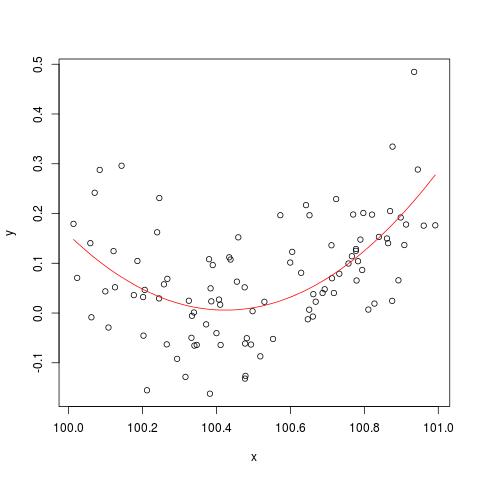
To illustrate the numerical stability issue mentioned by @cbeleites, here is an example from Simon Wood on how to "break" lm(). First we'll generate some simple data and fit a simple quadratic curve.
set.seed(1); n <- 100
xx <- sort(runif(n))
y <- .2*(xx-.5)+(xx-.5)^2 + rnorm(n)*.1
x <- xx+100
b <- lm(y ~ x+I(x^2))

plot(x,y)
lines(x, predict(b), col='red')

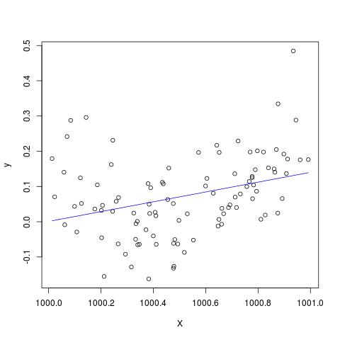
But if we add 900 to X, then the result should be pretty much the same except shifted to the right, no? Unfortunately not...
X <- x + 900
B <- lm(y ~ X+I(X^2))
plot(X,y)
lines(X, predict(B), col='blue')

Other algorithms can of course be "broken" in different ways with different examples.
