One way to study the problem would be some kind of GLM. For example, a Poisson or negative binomial regression with an intercept term and the $\{0,1\}$ variable for age is an obvious starting point. This model doesn't make any assumptions about how the age indicator variable is distributed, so it doesn't matter if it's heavily skewed in favor of younger or older workers. The coefficient estimate will tell you the direction and magnitude of age on the number of endorsements even if there's a disparity in workers' ages.
But a definitive reference for regression assumptions can be found inf Gleman and Hill, Data Analysis Using Regression and Multilevel/Hierarchical Models, section 3.6. All assumptions are listed in decreasing order of importance. The distribution of the independent variables doesn't appear on the list.
You write the that the researchers' response data were skewed. If the conditional expectation (the product $X\beta$ of the "true" model) of the response is non-normal (which skewness implies), then they are violating one of the key assumptions of OLS. A GLM may be a more appropriate model in that case, provided that the selected family and link function are correctly suited to the problem under study. Since the number of endorsements must be a non-negative positive integer, a normal model must be wrong because a normal model admits negative and non-integer values as valid numbers of endorsements.
Here's a demonstration using some fake data generated according to the process you describe. (The code is for R.) The data generation process fixes our parameter of interest $0.15$, and the intercept at $0.5$; this is the vector beta. Then we generate a binary indicator for the age variable that is $1$ only about 80% of the time; including an intercept, we have X. Then we generate the outcome y (endorsements) conditional on the expected value lambda.
set.seed(1969)
n   <- 2000
beta    <- c(0.5, .15)
X   <- cbind(rep(1, n), rbinom(n, size=1, prob=0.2))
lambda  <- exp(X%*%beta)
y   <- rpois(n, lambda=lambda)
summary(glm(y~0+X, family="poisson"(link=log)))
>    Estimate Std. Error z value Pr(>|z|)
X1  0.49279    0.01954  25.219  < 2e-16 ***
X2  0.17504    0.04079   4.291 1.78e-05 ***
As we can see, the model estimates the effect of age at roughly $0.17$, which is within 1 standard error of its true value, $0.15$.
But this doesn't necessarily mean that the study was done correctly. In my example, we precisely know the form of the data generating process, so it's very easy for us to re-create it. If there are other features influencing endorsements, then the authors' model suffers from omitted variable bias, and the coefficient estimates will be biased and inconsistent.
I suspect this regression, or some related variant, is what the researchers used. But this doesn't necessarily mean that the effect is as large as they stated (if it exists at all!). Perhaps the researchers selected the $35$ year age cut-off after examining the data, or any other kind of bias in the model construction step created the result ("The Garden of Forking Paths").
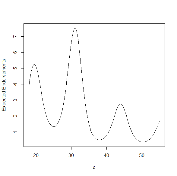
More subtly, it's possible that the trend is not binary at all but rather varies continuously and non-monotonically over one's life and is interactive with other worker characteristics. For example, it's possible that, as a function of age, there is some complex relationship as below. In this case, the estimates from the binary model will still be perfectly valid, but will not characterize well the kind of variation actually exists. A more flexible model, such as with splines, would be able to capture this.

