The quotes are from the link in the OP:
Identification of an AR model is often best done with the PACF.
For an AR model, the theoretical PACF “shuts off” past the order of the model. The phrase “shuts off” means that in theory the partial autocorrelations are equal to $0$ beyond that point. Put another way, the number of non-zero partial autocorrelations gives the order of the AR model. By the “order of the model” we mean the most extreme lag of x that is used as a predictor.
... a $k^{\text{th}}$ order autoregression, written as AR($k$), is a multiple linear regression in which the value of the series at any time t is a (linear) function of the values at times $t-1,t-2,\ldots,t-k:$
$$\begin{equation*} y_{t}=\beta_{0}+\beta_{1}y_{t-1}+\beta_{2}y_{t-2}+\cdots+\beta_{2}y_{t-k}+\epsilon_{t}. \end{equation*}$$
This equation looks like a regression model, as indicated on the linked paged... So what is a possible intuition...
In Chinese whispers or the telephone game as illustrated here
the message gets distorted as it is whispered from person to person, and the sentence is completely new after passing through two people. For instance, at time $t_2$ the message, i.e. "$\color{lime}{\small\text{CC}}$'s pool", is completely different in meaning from that at $t_o,$ i.e. "CV is cool!" The "correlation" that existed with $t_1$ ("$\color{lime}{\small\text{CC}}$ is cool!") in the word "$\color{lime}{\small\text{CC}}$" is gone; there are no remaining identical words, and even the intonation ("!") has changed.
This pattern repeats itself: there is a word shared at any given two consecutive time stamps, which goes away if $t_k$ is compared to $t_{k-2}.$
However, in this process of introducing errors at each step there is a similarity that spans further than just one single step: Although Chrisy's pool is different in meaning to CC is cool!, there is no denying their phonetic similarities or the rhyming of "pool" and "cool". Therefore it wouldn't be true that the correlation stops at $t_{k-1}.$ It does decay (exponentially) but it can be traced downstream for a long time: compare $t_5$ (Missi's cruel) to $t_0$ (CV is cool!) - there are still similarities.
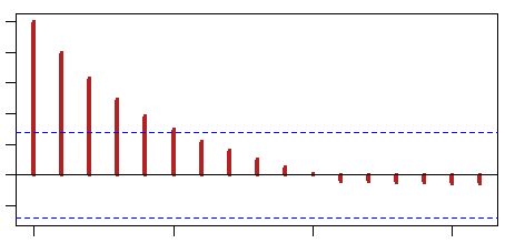
This explains the correlogram (ACF) in an AR($1$) processes (e.g. with coefficient $0.8$):
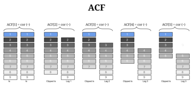
Multiple, progressively offset sequences are correlated, discarding any contribution of the intermediate steps. This would be the graph of the operations involved:
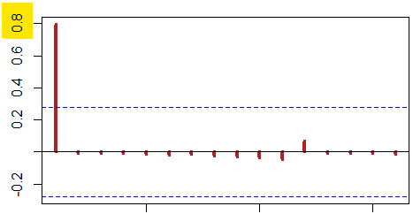
In this setting the PACF is useful in showing that once the effect of $t_{k-1}$ is controlled for, older timestamps than $t_{k-1}$ do not explain any of the remaining variance: all that remains is white noise:
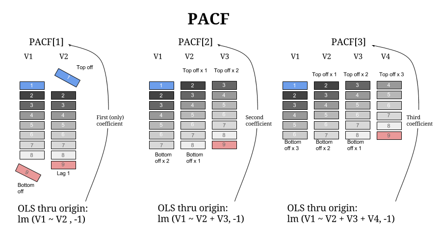
It is not difficult to come very close to the actual output of the R function by actually obtaining consecutive OLS regressions through the origin of farther lagged sequences, and collecting the coefficients into a vector. Schematically,
Identification of an MA model is often best done with the ACF rather than the PACF.
For an MA model, the theoretical PACF does not shut off, but instead tapers toward $0$ in some manner. A clearer pattern for an MA model is in the ACF. The ACF will have non-zero autocorrelations only at lags involved in the model.
A moving average term in a time series model is a past error (multiplied by a coefficient).
The $q^{\text{th}}$-order moving average model, denoted by MA($q$) is
$$x_t = \mu + w_t +\theta_1w_{t-1}+\theta_2w_{t-2}+\dots + \theta_qw_{t-q}$$
with $w_t \overset{\text{iid}}{\sim} N(0, \sigma^2_w).$
It turns out that the behavior of the ACF and the PACF are flipped compared to AR processes:
In the game above, $t_{k-1}$ was enough to explain all prior errors in transmitting the message (single significan bar in PACF plot), absorbing all prior errors, which had shaped the final message one error at a time. An alternative view of that AR($1$) process is as the addition of a long series of correlated mistakes (Koyck transformation), an MA($\infty$). Likewise, with some conditions, an MA($1$) process can be inverted into an AR($\infty$) process.
$$x_t = - \theta x_{t-1} - \theta^2 x_{t-2} - \theta^3 x_{t-3}+\cdots +\epsilon_t$$
The confusing part then is why the significant spikes in the ACF stop after the number of lags in MA($q$). But in an MA($1$) process the covariance is different from zero only at consecutive times $\small \text{Cov}(X_t,X_{t-1})=\theta \sigma^2,$ because only then the expansion $\small {\text{Cov}}(\epsilon_t + \theta \epsilon_{t-1}, \epsilon_{t-1} + \theta \epsilon_{t_2})=\theta \text{Cov}(\epsilon_{t-1}, \epsilon_{t-1})$ will result in a match in time stamps - all other combinations will be zero due to iid condition.
In the game of whispers, the error at $t_2$ (pool) is "correlated" with the value at $t_3$ (Chrissy's pool); however, there is no "correlation" between $t_3$ and the error at $t_1$ (CC).
Applying a PACF to a MA process will not result in "shut offs", but rather a progressive decay: controlling for the explanatory contribution of later random variables in the process does not render more distant ones insignificant as it was the case in AR processes.


