How should I interpret this residual plot?

Question

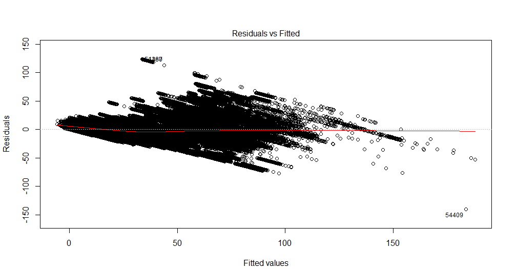
I am unable to interpret this graph. My dependent variable is total number of movie tickets that will be sold for a show. The independent variables are the number of days left before the show, seasonality dummy variables (day of week, month of year, holiday), price, tickets sold till date, movie rating, movie type (thriller, comedy, etc., as dummies). Also, please note that movie hall's capacity is fixed. That is, it can host maximum of x number of people only. I am creating a linear regression solution and it's not fitting my test data. So I thought of starting with regression diagnostics. The data are from a single movie hall for which I want to predict demand.

The is a multivariate dataset. For every date, there are 90 duplicate rows, representing days before the show. So, for 1 Jan 2016 there are 90 records. There is a 'lead_time' variable which gives me number of days before the show. So for 1 Jan 2016, if lead_time has value 5, it means it will have tickets sold until 5 days before the show date. In the dependent variable, total tickets sold, I will have the same value 90 times.

Also, as a side remark, is there any book that explains how to interpret residual plot and improve model afterwards?

Answer 1

The plot is very dense so it is not easy to see all trends there may be. You could run alternative tests for hetoroscedasticity and autocorrelation to get additional diagnostics.

What is visible is that over the first 100 values or so the variance of the residual increases which may hint to hetoroscedasticity. Afterwards the variance seems to decrease again. This somewhat non-linear behavior of the variance may also point to the need for a difference functional form (so maybe polynomial instead of linear). Another indication for this is the trend in residuals you observe in the high end of the fitted values (there aren't any positive residuals anymore).

Answer 2

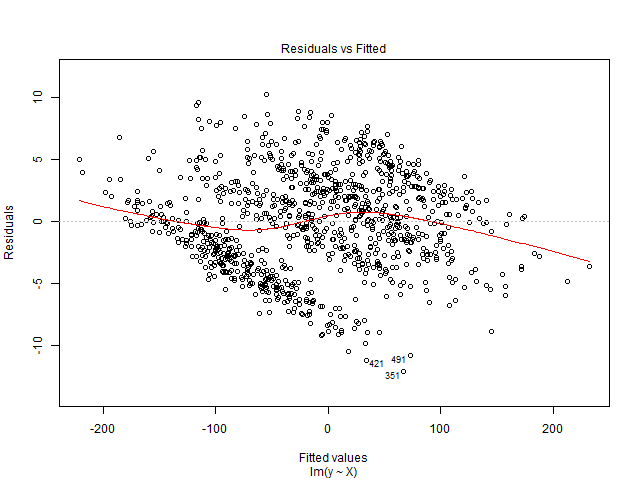
Your residual plot has a definite pattern, with several lines trending downward as fitted values increase. This pattern can occur if you fail to account for fixed/random effects in your model and the fixed effects are correlated with explanatory variables. Consider the following example:

set.seed(999)

N = 1000
num.groups = 10

alpha = runif(num.groups, -10, 10) #Fixed effects
beta = 10 #Slope parameter
group = sample(num.groups, N, replace = TRUE)

X = rnorm(N, mean = alpha[group], sd = 5) #Mean of X correlated with fixed effect
e = rnorm(N, sd = 1)
y = alpha[group] + X * beta + e

df = data.frame(group = as.factor(group), X, y)

m.no.fe = lm(y ~ X, data = df) #Not including group fixed effects
plot(m.no.fe, which = 1)

This results in the following residual/fitted plot:

You might see something similar if, for example, you regressed SAT scores on entry earnings for several high schools but failed to include high school fixed effects; each school will have different baseline earnings (i.e., fixed effects) and mean SAT scores, which are likely correlated.

Including group fixed effects, we get

m.fe = lm(y ~ group + X, data = df) #Now including fixed effects
plot(m.fe, which = 1)

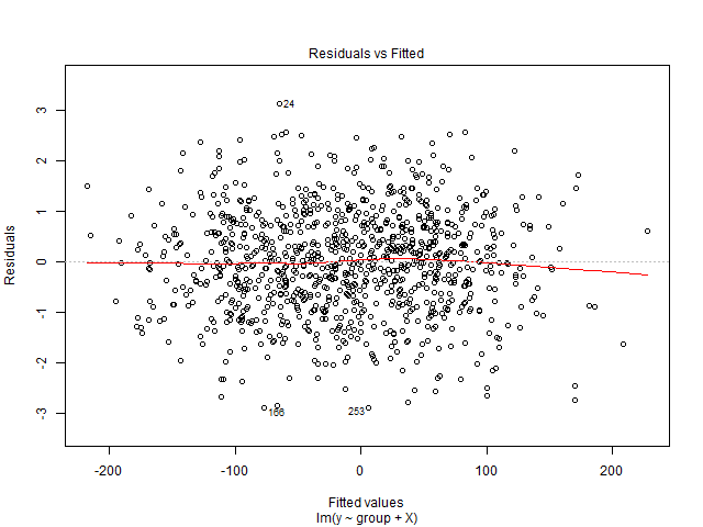
which gives a much better residual/fitted plot:

Answer 3

The residual plot does look unusual from the point of view of standard OLS (linear) regression. There is, for example, an indication of heteroscedasticity, specifically that the spread of the residuals is larger in the middle than at the two ends. This is not the real problem, however.

The real issue here is that you have fit the wrong model. OLS regression is based on the assumption that the response is normally distributed (conditional on the regressors—i.e., your $X$ variables). Your response is not normal, and cannot be. Your response is a number of seats sold out of a total number of seats in the theater. Your response is binomial. A binomial cannot be modeled correctly with OLS. You need to fit a logistic regression model.

There will be some additional issues you will need to address. A couple that are apparent from your description is that you have clustered observations, in the sense that you have multiple observations for the same show (i.e., over the 90 days). You need to address this non-independence, perhaps by fitting a GLMM. Another issue is that there will be a dependence between successive days within the same show. After all, if you have sold $y_d$ tickets on day $d$, you will have sold at least that many on day $d+1$. One way to try to address this is to fit only 89 days of data and to include the previous day's number as a covariate. (Sorry, on re-reading the question, I see you already have included a tickets sold till date variable.)

There may well be more issues to be addressed in modeling your data. These are fairly advanced topics; if you aren't familiar with them, you may need to work with a statistical consultant.