10
$\begingroup$

I have a 2D-histogram for two vectors, s1 and s2, generated using the hist3 function in Matlab:

[hist2D, binC] = hist3([s1' s2']);

I am normalizing it by making its total volume equal to unity, in the following manner:

L = binC{1}(2) - binC{1}(1);
B = binC{2}(2) - binC{2}(1);
totalVolume = sum(sum(hist2D.*L*B));
prob2D = hist2D/totalVolume;

Question: Is this correct way to normalize a 2D-histogram?

I have also normalized the 1D-histograms for s1 and s2, as shown below.

[hist1, binCentres1] = hist(s1);
binWidth1 = binCentres1(2) - binCentres1(1);
prob1 = hist1 / (sum(hist1) * binWidth1);
%same for s2

Question: How do I get the marginal (1D-)histograms from the normalized 2D-histogram?

I have tried doing this in the following manner:

prob1M = sum(prob2D, 2); %extract marginal for s1
prob2M = sum(prob2D, 1); %extract marginal for s2

If I were doing this correctly, I'd expect prob1 to be equal to prob1M. I seem to be on the right track because the bar graphs (below) look similar, but scaled on the vertical axis. Maybe I'm doing the normalizations wrong?
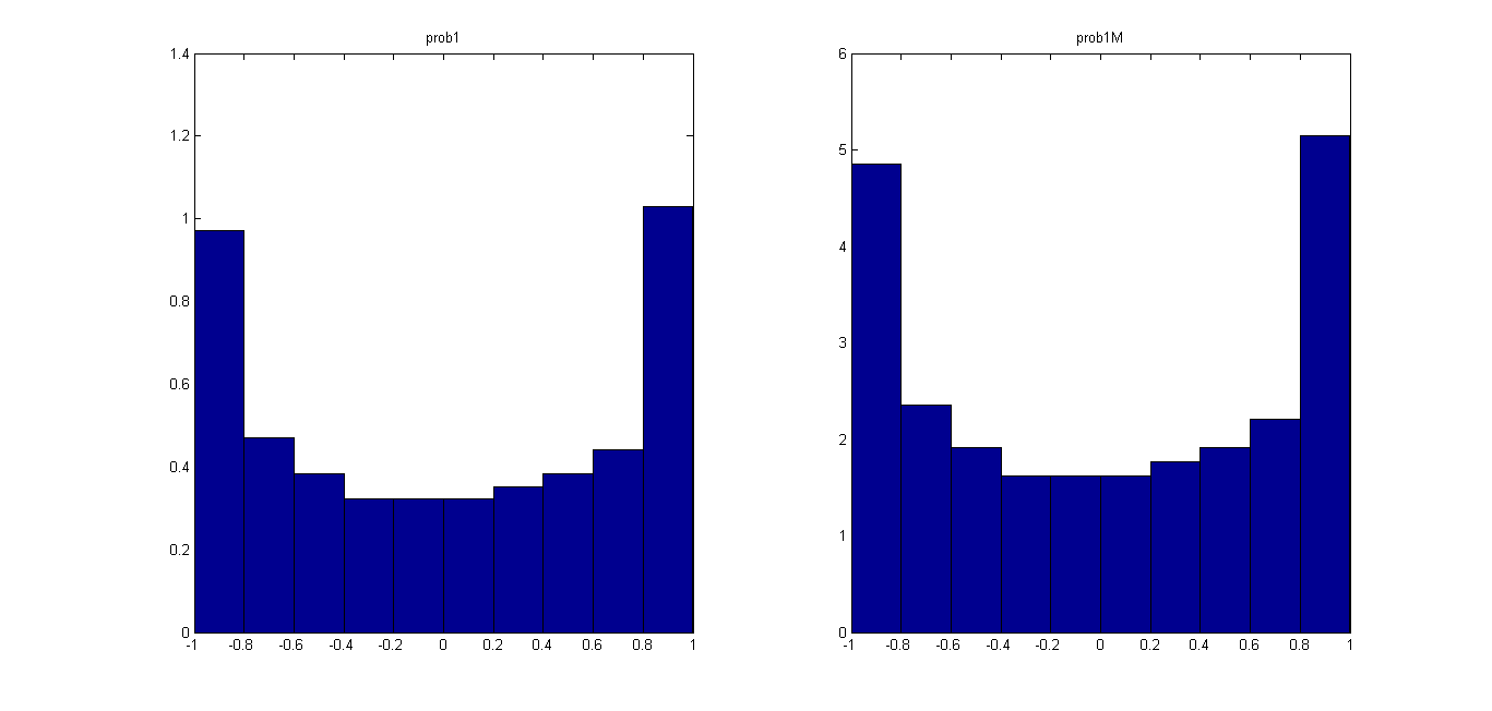
Bar Graphs fro prob1 and prob1M

I tried normalizing prob1M as well, using:

prob1M = prob1M / (sum(prob1M) * binWidth1);

Question: Is normalization still necessary if you get the marginals from a normalized 2D-histogram? Why / Why not?

After normalization, the area of prob1 and prob1M is equal to 1, where area is calculated as:

area = sum(binWidth1.*prob1)
%same for prob1M

However, prob1 and prob1M (and prob2 and prob2M) are still slightly different:

prob1 = 0.9412 0.4412 0.3235 0.3235 0.2941 0.3235 0.3235 0.4118 0.4706 1.1471
prob1M = 0.9706 0.4706 0.3824 0.3235 0.3235 0.3235 0.3530 0.3824 0.4412 1.0295

Thank you for your suggestions.

$\endgroup$

2 Answers 2

18
$\begingroup$

Densities can be hard to work with. Whenever you can, calculate with the total probabilities instead.

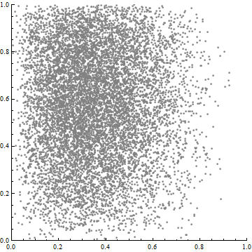
Usually, histograms begin with point data, such as these 10,000 points:

Scatterplot

A general 2D histogram tessellates the domain of the two variables (here, the unit square) by a collection $P$ of non-overlapping polygons (usually rectangles or triangles). To each polygon $p$ it assigns a density (probability or relative frequency per unit area). This is computed as

$$\text{density}(p) = \frac{\text{count within}(p)}{\text{total count}} / \text{area}(p).$$

The $\frac{\text{count within}(p)}{\text{total count}}$ part estimates the probability of $p$; when it is divided by the area of $p$, you get the density.

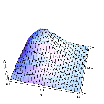
2D histogram

In this 2D histogram, the unit square has been tessellated by rectangles of width $1/26$ and height $1/11$.

2D histograms represent probability (or relative frequency) by means of volume: for each polygon $p$, the product of height and base, or density * area, returns $\frac{\text{count within}(p)}{\text{total count}}$. As a check, the total probability is obtained by summing the volumes over all polygons:

$$\eqalign{ \text{Total probability} &= \sum_{p \in P}\text{area}(p)\text{density}(p) \\ &= \sum_{p \in P}\frac{\text{count within}(p)}{\text{total count}} \\ &= \frac{1}{{\text{total count}}}\sum_{p \in P}\text{count within}(p) \\ &= \frac{\text{total count}}{\text{total count}}, }$$

which is equal to unity, as it should. (In the previous image, the histogram heights range from $0$ almost up to $3$; the total volume is $1$.)

To get a marginal density--say, along the x-axis--you slice that axis into bins at cutpoints $x_0 \lt x_1 \lt x_2 \lt \cdots \lt x_n$. (These are allowed to have unequal lengths.) Each bin $(x_i, x_{i+1}]$ determines a vertical slice of the 2D region (consisting of all points $(x,y)$ for which $x_i \lt x \le x_{i+1}$). Let's call this strip $S_i$. As with any (1D) histogram, compute (or estimate) the total probability within each bin and divide by the bin width to obtain the histogram value. The total probability is usually estimated as the the sum of probabilities in polygons intersecting that strip:

$$\Pr[x_i\lt x \le x_{i+1}] = \sum_{p \in P}\text{area}(p\cap S_i)\text{density}(p).$$

Dividing this value by $x_{i+1} - x_i$ gives the value for the histogram of the marginal distribution. Repeat for each bin.

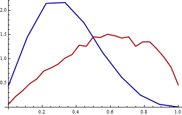
Marginals

The x-marginal histogram is in blue and the y-marginal histogram is in red. Each has a total area of $1$.

$\endgroup$
0
2
$\begingroup$

If you normalize a histogram, you don't need to take the bin-width into account. You can look at it like this: When estimating a histogram from continuous data, you basically discretize it first (by setting each value to the bin center which is closest to it) and then generate a discrete histogram for the discretized data. This is simply normalized by dividing by the sum over all its elements.

When taking the bin-width into account you are essentially not estimating a histogram anymore, but a piecewise constant approximation to the density. If you do that, then you also have to take the bin-width into account for marginalizing. This means your code for the marginals needs to be

prob1M = sum(prob2D, 2)*L;

Edit: Histogram, discrete probability distribution, density

Since there seems to be some confusion about histograms, I try to make it clearer.

Let's first look at discrete data, e.g. integers from 1 to 10. When you observe $m$ samples from a random variable that takes values between 1 and 10 you can build a histogram. If you normalize that histogram (by dividing it by $m$), you get a discrete probability distribution $p_1,...,p_{10}$. There is no bin width involved, since discrete probability distributions are normalized by summing, i.e. $\sum_{i=1}^{10}p_i = 1$.

When you bin continuous data, what you really do is to (1) discretize it first and (2) bin it. Let's say, we have $m$ samples of a random variable $X$ that takes on values in $[0,10]$. When building a histogram, we first map each value to the nearest bin center, i.e. $1.34$ gets mapped to $1.5$, $0.1$ gets mapped to $0.5$, and so on. Afterwards, we again build a histogram an normalize it. However, now the histogram values have a different meaning. For example, when we look at the first bin for values between $0$ and $1$, then this contains all the probability of the values $X$ that end up in that bin, i.e. if $q$ is the true underlying density, then $p_{1} = \int_0^1 q(x) dx$. Therefore, you the value of the normalized histogram already implicitly contains the bin-width. Furthermore, there is really nothing to integrate, since the histogram runs again over discrete values, i.e. $0.5, 1.5, ..., 9.5$.

Now, if you want to use the histogram to get a continuous density, one that integrates to one, the you need to take into account the bin width. You can do that by defining $$p(x) = \sum_{i=1}^{10} \frac{p_i}{\Delta} \cdot I_i.$$

$I_i$ is a function that is one on the $i$th bin and zero otherwise. $\Delta$ is the bin width which would be $\Delta = 1$ in our example. This function integrates to one. For our example $$\int_0^{10} p(x) dx = \int_0^{10} \sum_{i=1}^{10} \frac{p_i}{\Delta} \cdot I_i dx = \sum_{i=1}^{10} \frac{p_i}{\Delta} \cdot \underbrace{\int_0^{10} \sum_{i=1}^{10} I_i dx}_{=\Delta} = \sum_{i=1}^{10} p_i = 1. $$

What this does is to approximate the true density by a pieceswise constant function.

If you want to estimate mutual information, you can use the histogram values itself, without bin-width. For a continuous density you have $p_i = \int_{ith\:bin} q(x)dx = \Delta \cdot \xi_i$ where $\xi_i$ is a value from the bin such that the equality holds. Since you can write it as a product, the bin-width in the quotient cancels and the sum converges to the Riemann integral for the mutual information.

$\endgroup$
9
  • $\begingroup$ Thank you. Some questions: Wouldn't taking the bin-width into account make the approximation more accurate? Or am I wrong? And even if I do NOT take the bin width into account (as you suggested) - i.e. prob1 = hist1 / (sum(hist1)); - prob1 and prob1M still differ by a fraction (similar to the normalized ones shown in the question). $\endgroup$
    – Rachel
    Commented Mar 13, 2012 at 17:28
  • $\begingroup$ have you checked whether the bin locations are the same? $\endgroup$
    – fabee
    Commented Mar 13, 2012 at 17:45
  • $\begingroup$ Concerning your other question: The bin width does not make the estimate more accurate (it's just a factor), but it changes what the histogram means. Without the bin-width it is just a histogram over discrete values, like a discrete probability distribution (if normalized). With the bin-width you treat is as a piecewise constant continuous probability density. For your other question with the MI, it does not make a difference whether you take into account the bin-width or not (since it cancles in the quotient). For differential entropy estimation, however, it does. There you need the bin-width $\endgroup$
    – fabee
    Commented Mar 13, 2012 at 17:50
  • 1
    $\begingroup$ I find this discussion confusing, because by definition a histogram represents probability by area. Therefore it must be "normalized" in the sense that the total of the bar areas must equal unity. (Anything else is just a frequency (or probability) bar chart.) The answers to this set of questions follow easily from the definition. $\endgroup$
    – whuber
    Commented Mar 13, 2012 at 18:18
  • $\begingroup$ @whuber I thought so to, that's why I tried to normalize in such a way that the area/volume for the 1D/2D-histograms (respectively) is equal to unity. It seems that both methods of normalization are used, and now I'm even more confused! I need the normalized versions to calculate the Mutual Information. $\endgroup$
    – Rachel
    Commented Mar 13, 2012 at 19:48

Your Answer

By clicking “Post Your Answer”, you agree to our terms of service and acknowledge you have read our privacy policy.

Not the answer you're looking for? Browse other questions tagged or ask your own question.