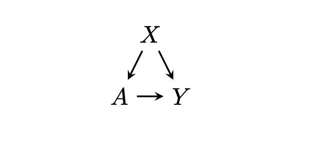
Causal Inference is an important topic in statistics generally, for both observational research and controlled experiments such as clinical trials.
A DAG is a Directed Acyclic Graph.
A “Graph” is a structure with nodes (which are usually variables in statistics) and arcs (lines) connecting nodes to other nodes. “Directed” means that all the arcs have a direction, where one end of the arc has an arrow head, and the other does not, which usually refers to causation. “Acyclic” means that the graph is not cyclic – that means there can be no path from any node that leads back to the same node. In statistics a DAG is a very powerful tool to aid in causal inference – to estimate the causal effect of one variable (often called the main exposure) on another (often called the outcome) in the presence of other variables which may be competing exposures, confounders or mediators. The DAG can be used to identify a minimal sufficient set of variables to be used in a multivariable regression model for the estimation of said causal effect. For example it is usually a very bad idea to condition on a mediator (a variable that lies on the causal path between the main exposure and the outcome), while it is usually a very good idea to condition on a confounder (a variable that is a cause, or a proxy for a cause, of both the main exposure and the outcome). It is also a bad idea to condition on a collider (to be defined below).
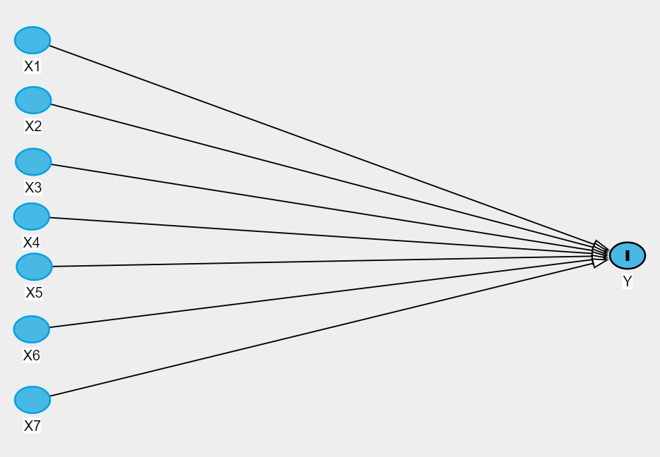
But first, what is the problem we want to overcome? This is what a multivariable regression model looks like to your statistical software:

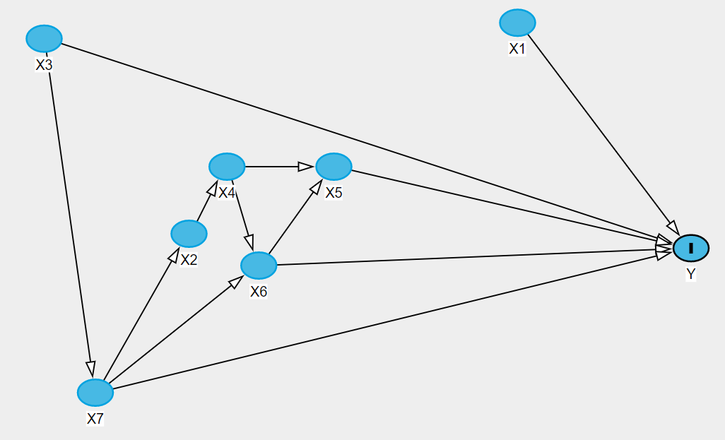
The software does not “know” which variables are our main exposure, competing exposures, confounders or mediators. It treats them all the same. In the real world it is far more common for the variables to be inter-related. For example, knowledge of the particular area of research may indicate a structure such as:

It is the responsibility of the researchers to determine the causal pathways by utilising their expertise in the relevant subject matter. DAGs are graphical representations of a collection of causal ideas that are typically abstracted and relevant to certain causal relationships. It is not unusual for one researcher's DAG to differ from another researcher's DAG. Similarly, a researcher may develop several DAGs for the same study design. Employing DAGs in a systematic manner, as I will try to show below, serves as a means to acquire knowledge or substantiate a certain theory.
Let’s suppose that our primary interest is in the causal effect of $X7$ on $Y$. What are we to do? A very naive approach is simply to put all the variables into a regression model, and take the estimated coefficient for $X7$ as our “answer”. This would be a big mistake. It turns out that the only variable that should be adjusted for in this DAG is $X3$, because it is a confounder. But what if our interest was in the effect of $X3$, not $X7$ ? Do we simply use the same model (also containing $X7$) and just take the estimate of $X3$ as our “answer”? No! In this case, we do not adjust for $X7$ because it is a mediator. No adjustment is needed at all. In both cases, we may also adjust for $X1$ because this is a competing exposure and will improve the precision of our casual inferences in both models. In both models we should not adjust for $X2$, $X4$, $X5$ and $X6$ because all of them are mediators for the effect of $X7$ on $Y$.
So, getting back to the question, how do DAGs actually enable us to do this? First we need to establish a few ground truths.
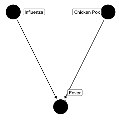
A collider is a variable which has more than 1 cause – that is, at least 2 arrows are pointing at it (hence the incoming arrows “collide”). $X5$ in the above DAG is a collider
If there are no variables being conditioned on, a path is blocked if and only if it contains a collider. The path $X4 \rightarrow X5 \leftarrow X6$ is blocked by the collider $X5$.
Note: when we talk about "conditioning" on a variable this could refer to a few things, for example stratifying, but perhaps more commonly including the variable as a covariate in a multivariable regression model. Other synonymous terms are "controlling for" and "adjusting for".
Any path that contains a non-collider that has been conditioned on is blocked. The path $Y \leftarrow X3 \rightarrow X7$ will be blocked if we condition on $X3$.
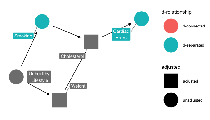
A collider (or a descendant of a collider) that has been conditioned on does not block a path. If we condition on $X5$ we will open the path $X4 \rightarrow X5 \leftarrow X6$
A backdoor path is a non-causal path between an outcome and a cause. It is non-causal because it contains an arrow pointing at both the cause and the outcome. For example the path $Y \leftarrow X3 \rightarrow X7$ is a backdoor path from $Y$ to $X3$.
Confounding of a causal path occurs where a common cause for both variables is present. In other words confounding occurs where an unblocked backdoor path is present. Again, $Y \leftarrow X3 \rightarrow X7$ is such a path.
So, armed with this knowledge, let’s see how DAGs help us with removing bias:
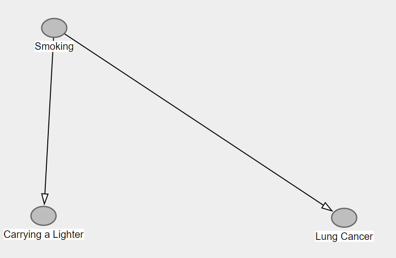
The definition of confounding is 6 above. If we apply 4 and condition on the confounder we will block the backdoor path from the outcome to the cause, thereby removing confounding bias. The example is the association of carrying a lighter and lung cancer:

Carrying a lighter has no causal effect on lung cancer, however, they share a common cause - smoking - so applying rule 5 above, a backdoor path from Lung cancer to carrying a lighter is present which induces an association between carrying a lighter and Lung cancer. Conditioning on Smoking will remove this association, which can be demonstrate with a simple simulation where I use continuous variables for simplicity:
> set.seed(15)
> N       <- 100
> Smoking <- rnorm(N, 10, 2)
> Cancer  <- Smoking + rnorm(N)
> Lighter <- Smoking + rnorm(N)

> summary(lm(Cancer ~ Lighter))

Coefficients:
      Estimate Std. Error t value Pr(>|t|)
(Intercept)  0.66263    0.76079   0.871    0.386
Lighter      0.91076    0.07217  12.620   <2e-16 ***
which shows the spurious association between Lighter and Cancer, but now when we condition on Smoking:
> summary(lm(Cancer ~ Lighter + Smoking))

Coefficients:
            Estimate Std. Error t value Pr(>|t|)
(Intercept) -0.42978    0.60363  -0.712    0.478
Lighter      0.07781    0.11627   0.669    0.505
Smoking      0.95215    0.11658   8.168 1.18e-12 ***
...the bias is removed.
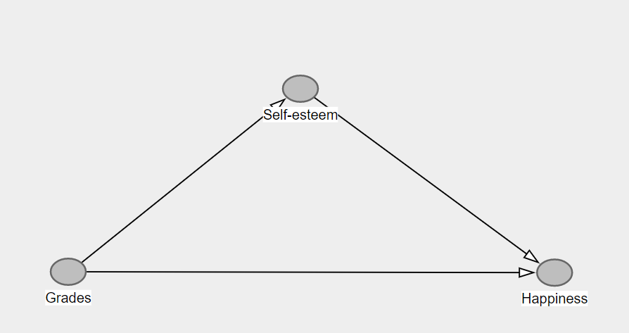
A mediator is a variable that lies on the causal path between the cause and the outcome. This means that the outcome is a collider. Therefore, applying rule 3 means that we should not condition on the mediator otherwise the indirect effect of the cause on the outcome (i.e., that mediated by the mediator) will be blocked. A good example example is the grades of a student and their happiness. A mediating variable is self-esteem:

Here, Grades has a direct effect on Happiness, but it also has an indirect effect mediated by self-esteem. We want to estimate the total causal effect of Grades on Happiness. Rule 3 says that a path that contains a non-collider that has been conditioned on is blocked. Since we want the total effect (i.e., including the indirect effect) we should not condition on self-esteem otherwise the mediated path will be blocked, as we can see in the following simulation:
> set.seed(15)
> N          <- 100
> Grades     <- rnorm(N, 10, 2)
> SelfEsteem <- Grades + rnorm(N)
> Happiness  <- Grades + SelfEsteem + rnorm(N)
So the total effect should be 2:
> summary(m0 <- lm(Happiness ~ Grades)) # happy times

Coefficients:
            Estimate Std. Error t value Pr(>|t|)
(Intercept)  1.05650    0.79509   1.329    0.187
Grades       1.90003    0.07649  24.840   <2e-16 ***
which is what we do find. But if we now condition on self esteem:
> summary(m0 <- lm(Happiness ~ Grades + SelfEsteem

Coefficients:
            Estimate Std. Error t value Pr(>|t|)
(Intercept)  1.39804    0.50783   2.753  0.00705 **
Grades       0.81917    0.10244   7.997 2.73e-12 ***
SelfEsteem   1.05907    0.08826  11.999  < 2e-16 ***
only the direct effect for grades is estimated, due to blocking the indirect effect by conditioning on the mediator SelfEsteem.
This is probably the most difficult one to understand, but with the aid of a very simple DAG we can easily see the problem:

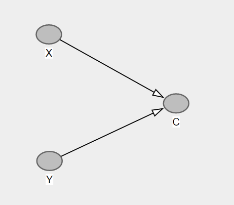
Here, there is no causal path between X and Y. However, both cause C, the collider. If we condition on C, then applying rule 4 above we will invoke collider bias by opening up the (non causal) path between X, and Y. This may be a little hard to grasp at first, but it should become apparent by thinking in terms of equations. We have X + Y = C. Let X and Y be binary variables taking the values 1 or zero. Hence, C can only take the values of 0, 1 or 2. Now, when we condition on C we fix its value. Say we fix it at 1. This immediately means that if X is zero then Y must be 1, and if Y is zero then X must be one. That is, X = -Y, so they are perfectly (negatively) correlated, conditional on C= 1. We can also see this in action with the following simulation:
> set.seed(16)
> N <- 100
> X <- rnorm(N, 10, 2)
> Y <- rnorm(N, 15, 3)
> C <- X + Y + rnorm(N)
So, X and Y are independent so we should find no association:
> summary(m0 <- lm(Y ~ X))

Coefficients:
            Estimate Std. Error t value Pr(>|t|)
(Intercept) 14.18496    1.54838   9.161 8.01e-15 ***
X            0.08604    0.15009   0.573    0.568
and indeed no association is found. But now condition on C
> summary(m1 <- lm(Y ~ X + C))

Coefficients:
            Estimate Std. Error t value Pr(>|t|)
(Intercept)  1.10461    0.61206   1.805   0.0742 .
X           -0.92633    0.05435 -17.043   <2e-16 ***
C            0.92454    0.02881  32.092   <2e-16 ***
and now we have a spurious association between X and Y.
Now let’s consider a slightly more complex situation:

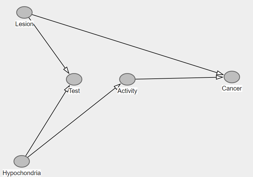
Here we are interested in the causal effect of Activity on Cervical Cancer. Hypochondria is an unmeasured variable which is a psychological condition that is characterized by fears of minor and sometimes non-existent medical symptoms being an indication of major illness. Lesion is also an unobserved variable that indicates the presence of a pre-cancerous lesion. Test is a diagnostic test for early stage cervical cancer. Here we hypothesise that both the unmeasured variables affect Test, obviously in the case of Lesion, and by making frequent visits to the doctor in the case of Hypochondria. Lesion also (obviously causes Cancer) and Hypochondria causes more physical activity (because persons with hypochondria are worried about a sedentary lifestyle leading to disease in later life.
First notice that if the collider, Test, was removed and replace with an arc either from Lesion to Hypochondria or vice versa, then our causal path of interest, Activity to Cancer, would be confounded, but due to rule 2 above, the collider blocks the backdoor path $\text{Cancer}\leftarrow \text{Lesion} \rightarrow \text{Test} \leftarrow \text{Hypochondria} \rightarrow \text{Activity}$, as we can see with a simple simulation:
> set.seed(16)
> N            <- 100
> Lesion       <- rnorm(N, 10, 2)
> Hypochondria <- rnorm(N, 10, 2)
> Test         <- Lesion + Hypochondria + rnorm(N)
> Activity     <- Hypochondria + rnorm(N)
> Cancer       <- Lesion + 0.25 * Activity + rnorm(N)
where we hypothesize a much smaller effect of Activity on Cancer than Lesion on Cancer
> summary(lm(Cancer ~ Activity))

    Coefficients:
            Estimate Std. Error t value Pr(>|t|)
(Intercept) 10.47570    1.01150  10.357   <2e-16 ***
Activity     0.21103    0.09667   2.183   0.0314 *
And indeed we obtain a reasonable estimate.
Now, also observe the association of Activity and Cancer with Test (due to their common, but unmeasured causes:
> cor(Test, Activity); cor(Test, Cancer)
[1] 0.6245565
[1] 0.7200811
The traditional definition of confounding is that a confounder is variable that is associated with both the exposure and the outcome. So, we might mistakenly think that Test is a confounder and condition on it. However, we then open up the backdoor path $\text{Cancer}\leftarrow \text{Lesion} \rightarrow \text{Test} \leftarrow \text{Hypochondria} \rightarrow \text{Activity}$, and introduce confounding which would otherwise not be present, as we can see from:
> summary(lm(Cancer ~ Activity + Test))

Coefficients:
            Estimate Std. Error t value Pr(>|t|)
(Intercept)  1.77204    0.98383   1.801   0.0748 .
Activity    -0.37663    0.07971  -4.725 7.78e-06 ***
Test         0.72716    0.06160  11.804  < 2e-16 ***
Now not only is the estimate for Activity biased, but it is of larger magnitude and of the opposite sign!
The preceding example can also be used to demonstrate selection bias. A researcher may identify Test as a potential confounder, and then only conduct the analysis on those that have tested negative (or positive).
> dtPos <- data.frame(Lesion, Hypochondria, Test, Activity, Cancer)
> dtNeg <- dtPos[dtPos$Test <  22, ]
> dtPos <- dtPos[dtPos$Test >= 22, ]
> summary(lm(Cancer ~ Activity, data = dtPos))

Coefficients:
            Estimate Std. Error t value Pr(>|t|)
(Intercept) 13.15915    3.07604   4.278 0.000242 ***
Activity     0.08662    0.25074   0.345 0.732637
So for those that test positive we obtain a very small positive effect, that is not statistically significant at the 5% level
> summary(lm(Cancer ~ Activity, data = dtNeg))

    Coefficients:
            Estimate Std. Error t value Pr(>|t|)
(Intercept) 12.18865    1.12071  10.876   <2e-16 ***
Activity    -0.01553    0.11541  -0.135    0.893
And for those that test negative we obtain a very small negative association which is also not significant.

