The statistic Cohen's d follows a scaled non-central t-distribution.
This statistic is the difference of the mean divided by an estimate of the sample standard deviation of the data:
$$d = \frac{\bar{x}_1-\bar{x}_2}{\hat{\sigma}}$$
It is used in power analysis and relates to the t-statistic (which is used in significance testing)
$$d = n^{-0.5} t $$
This factor $n$ is computed as $n=\frac{n_1 n_2}{n_1+n_2}$
The difference is that
- to compute $d$ we divide by the standard deviation to the data
- and for $t$ we divide by the standard error of the means
(and these differ by a factor $\sqrt{n}$)
Confidence interval based on normal approximation of non-central t-distribution
The articles that you mention relate to the article Larry V. Hedges 1981 "Distribution Theory for Glass's Estimator of Effect Size and Related Estimators"
There they give a large sample approximation of Cohen's d as a normal distribution with the mean equal to $d$ and the variance equal to $$\frac{n_1 + n_2}{n_1n_2} + \frac{d^2}{2(n_1+n_2)}$$
These expressions stem from the mean and variance of the non-central t-distribution. For the variance we have:
$$\begin{array}{crl}
\text{Var}(t) &=& \frac{\nu(1+\mu^2)}{\nu-2} - \frac{\mu^2 \nu}{2} \left(\frac{\Gamma((\nu-1)/2)}{\Gamma(\nu/2)}\right)^2 \\ &\approx& \frac{\nu(1+\mu^2)}{\nu-2} - \frac{\mu^2 \nu}{2} \left(1- \frac{3}{4\nu-1} \right)^{-2} \end{array} $$
Where $\nu = n_1+n_2-2$ and $\mu = d \sqrt{\frac{n_1n_2}{n_1+n_2}}$. For cohen's d this is multiplied with ${\frac{n_1+n_2}{n_1n_2}}$
$$\text{Var}(d) = \frac{n_1+n_2}{n_1n_2} \frac{\nu}{\nu-2} + d^2 \left( \frac{\nu}{\nu-2} -\frac{1}{(1-3/(4\nu-1))^2} \right)$$
The variations in the three formula's that you mention are due to differences in simplifications like $\nu/(\nu-2) \approx 1$ or $\nu = n_1+n_2-2 \approx n_1+n_2$.
In the most simple terms
$$\frac{\nu}{\nu-2} = 1 + \frac{2}{\nu-2} \approx 1$$
and (using a Laurent Series)
$$\frac{\nu}{\nu-2} -\frac{1}{(1-3/(4\nu-1))^2} = \frac{1}{2\nu} + \frac{31}{16\nu^3} + \frac{43}{8\nu^3} + \dots \approx \frac{1}{2\nu} \approx \frac{1}{2(n_1 + n_2)} $$
Which will give
$$\text{Var}(d) \approx \frac{n_1+n_2}{n_1n_2} + d^2\frac{1}{2(n_1+n_2)} $$
Confidence interval based on computation
If you would like to compute the confidence interval more exactly then you could compute those values of the non-central t-distribution for which the observed statistic is an outlier.
Example code:
### input: observed d and sample sizes n1 n2
d_obs = 0.1
n1 = 5
n2 = 5

### computing scale factor n and degrees of freedom
n  = n1*n2/(n1+n2)
nu = n1+n2-2


### a suitable grid 'ds' for a grid search
### based on
var_est <- n^-1 + d_obs^2/2/nu
ds <- seq(d_obs-4*var_est^0.5,d_obs+4*var_est^0.5,var_est^0.5/10^4)


### boundaries based on limits of t-distributions with ncp parameter
### for which the observed d will be in the 2.5% left or right tail
upper <- min(ds[which(pt(d_obs*sqrt(n),nu,ds*sqrt(n))<0.025)])*sqrt(n)    # t-distribution boundary
upper/sqrt(n)                                                             # scaled boundary
lower <- max(ds[which(pt(d_obs*sqrt(n),nu,ds*sqrt(n))>0.975)])*sqrt(n)
lower/sqrt(n)
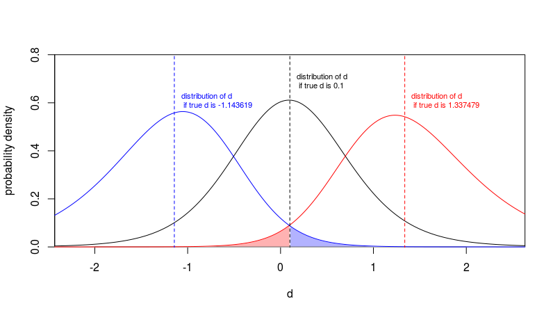
Below is a situation for the case when the observed $d$ is 0.1 and the sample sizes are $n_1 = n_2 = 5$. In this case the confidence interval is
$$CI: -1.43619,1.337479$$
In the image you see how $d$ is distributed for different true values of $d$ (these distributions are scaled non-central t-distributions).
The red curve is the distribution of observed $d$ if the true value of $d$ would be equal to the upper limit of the confidence interval $1.337479$. In that case the observation of $d=0.1$ or lower would only occur in 2.5% of the cases (the red shaded area).
The blue curve is the distribution of the observed $d$ if the true value of $d$ would be equal to the lower limit of the confidence interval $-1.143619$. In that case the observation of $d=0.1$ or higher would only occur in 2.5% of the cases (the blue shaded area).


