To estimate confidence intervals we could use simulations of the distribution of the biggest difference of the mean when we place half the means on one end and the other half on the other end.
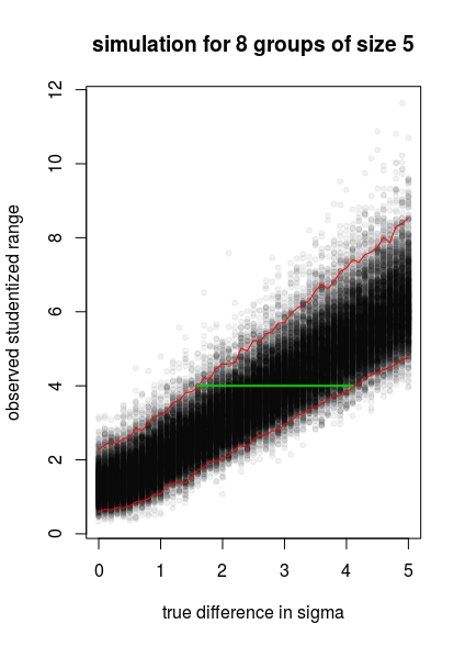
It would look for instance like this.

Then based on some observed range you can compute which boundaries associate with that, and make your confidence interval.
In the example image, a demonstration is given for the case that the observed studentized range would be 4 with a green line that corresponds to an estimate of a 95% confidence interval. The line is between the red lines, which give the upper and lower 2.5% of the samples.
A few more things need to be done:
- We used only the range and compute a worst case for the distribution of the range when all the groups are at the furthest edges. This does not use all the information. When only two means are very far away and the rest is in the middle then this is a different situation from when many means are at the edges.
- We used a simulation but it would be nice if some expression would be used. This is not so easy. The case for the situation that all the means are equal is the studentized range distribution. That is already difficult to compute, and now you need a generalization of it.
computer code for the image
### nu = number in sample
### nl = number of samples in each left side
### d = distance between means
### nr = number of samples in right side
### m = number of samples in the middle
### d2 = position of the middle samples

simdif = function(nu, nl, d, nr = nl, m = 0, d2 = d/2) {
  ### means of the different groups
  mean = c(rep(0,nl),rep(d2,m),rep(d,nr))

  ### compute samples
  x = matrix(rnorm(nu*(nl+m+nr),mean = mean), nu, byrow = 1)

  ### compute sample means
  mu = colMeans(x)

  ### compute pooled sample variance
  RSS = sum((x - rep(1,nu) %*% t(as.matrix(mu)))^2)
  sig = sqrt(RSS/(nu*(nl+m+nr)-nu))

  ### studentized range
  range = (max(mu)-min(mu))/sig

  return(range)
}


### compute for different distances
dv = seq(0,5,0.1)

### smp contains the simulation
smp = c()
### pct975 stores the upper 97.5-th quantile
### pct025 stores the lower 2.5-th quantile
pct975 = c()
pct025 = c()

### do the sampling
nrep = 10^3
set.seed(1)
for (di in dv) {
  sample = replicate(nrep, simdif(5,4,di))
  perc = quantile(sample, probs = c(0.025,0.975))
  smp = cbind(smp,sample)
  pct975 = c(pct975,perc[2])
  pct025 = c(pct025,perc[1])
}

dcor = rep(1,nrep) %*% t(as.matrix(dv))

### plot experimental distribution with confidence boundaries
plot(dcor, smp, pch = 21, col = rgb(0,0,0,0.05), bg = rgb(0,0,0,0.05), cex = 0.7,
     main = "simulation for 8 groups of size 5",
     ylab = "observed studentized range",
     xlab = "true difference in sigma")
lines(dv,pct975, col = 2)
lines(dv,pct025, col = 2)

### example confidence interval
c1 = which.min(abs(pct975-4))
c2 = which.min(abs(pct025-4))
lines(dv[c(c1,c2)], c(4,4), col = 3, lwd = 4, lty = 2)
Edit:
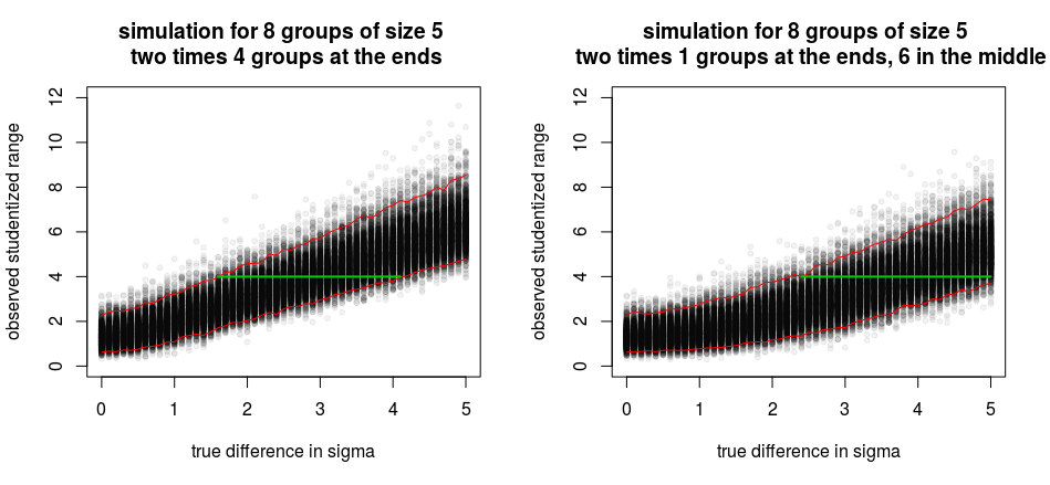
I notice a problem with my approach. I looked at the situation of the 8 groups split up into two times 4 groups at the extreme ends. This gives a larger range than other configurations. But that is only good to compute the upper limit and would be good for a one-sided confidence interval. For the lower boundary, we should not look at the worst-case but at the least worse case. That is when only 2 out of the 8 groups are at the far ends and the rest is exactly in the middle.
The code above already anticipated this possibility to compute the least worse case. With the code above we would use simdif(5,1,di,1,6) (which places 1 group mean at the lower end, 1 group mean on the upper end, and the other 6 in the middle) instead of simdif(5,4,di,4,0). Then we will see lower values for the range and the confidence interval boundaries shift to the right (higher values).
So, with this approach, we would need to combine those intervals. It is a bit the curse of the composite null hypothesis. We need to cover the multiple situations that correspond with the null hypothesis.

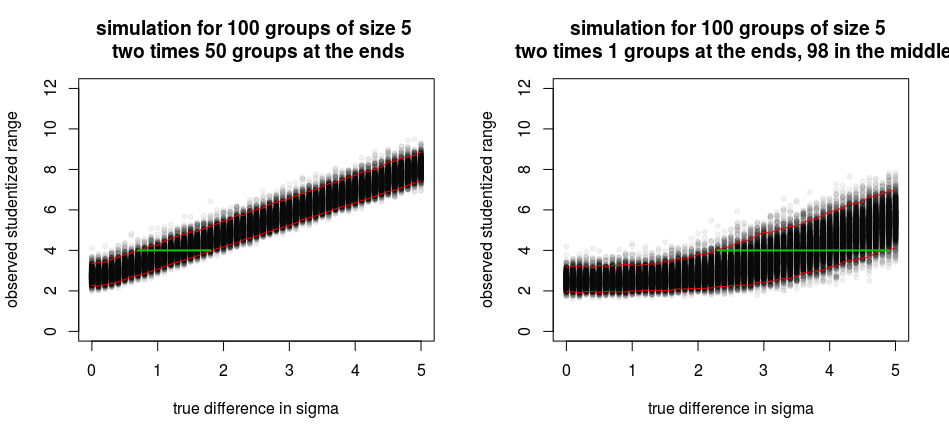
The effect of different configurations becomes even more extreme when we are comparing more group means. In the image below we look at the distribution of the range of 100 group means. In the left image, the distribution is computed for two times 50 groups with the mean on the ends. In the right image, there are only two times one group with the mean at the end, and the rest is in the middle. In the left image, the range is much larger. The limits for the confidence interval are very far from each other. This means that it would be useful to incorporate more data than just the range, and I should not should have ignored the distribution of the other 98 groups.
