Residuals pattern in Cox proportional hazards model

Question

I do a survival regression on some time-to-event data (vehicle breakdowns) with some covariates (essentially the age of the vehicle and some boolean variables for vehicle type). I must admit that I am not so sure about the quality of the data and whether they result from multiple processes instead of one.

For the implementation, I use the Python package lifelines and the CoxPH fitter in particular.

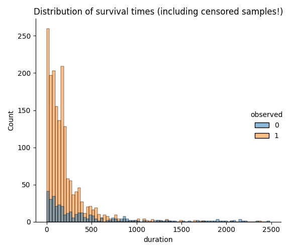
This is the distribution of survival times in my data (for both censored and non-censored points!):

Here is the model summary:

<lifelines.CoxPHFitter: fitted with 2081 total observations, 354 right-censored observations>
             duration col = 'duration'
                event col = 'observed'
              cluster col = 'vehicle'
          robust variance = True
      baseline estimation = breslow
   number of observations = 2081
number of events observed = 1727
   partial log-likelihood = -11593.48
         time fit was run = 2023-03-18 06:32:51 UTC

---
                               coef  exp(coef)   se(coef)   coef lower 95%   coef upper 95%  exp(coef) lower 95%  exp(coef) upper 95%
covariate
year_of_manufacture            0.05       1.06       0.01             0.03             0.08                 1.03                 1.08
N7411   0.90       2.46       0.18             0.54             1.26                 1.72                 3.52
N7412   1.25       3.50       0.18             0.91             1.60                 2.48                 4.94
N7413   1.13       3.11       0.17             0.80             1.46                 2.24                 4.31
N7460  -0.47       0.63       0.33            -1.12             0.19                 0.33                 1.21
N7440   0.76       2.14       0.20             0.38             1.14                 1.46                 3.13

                               cmp to     z      p   -log2(p)
covariate
year_of_manufacture              0.00  4.15 <0.005      14.86
N7411     0.00  4.95 <0.005      20.33
N7412     0.00  7.11 <0.005      39.68
N7413     0.00  6.76 <0.005      36.06
N7460     0.00 -1.39   0.16       2.61
N7440     0.00  3.89 <0.005      13.28
---
Concordance = 0.56
Partial AIC = 23198.95
log-likelihood ratio test = 163.41 on 6 df
-log2(p) of ll-ratio test = 106.14

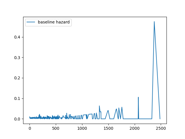
This is how the modeled baseline hazard looks:

I now have some questions:

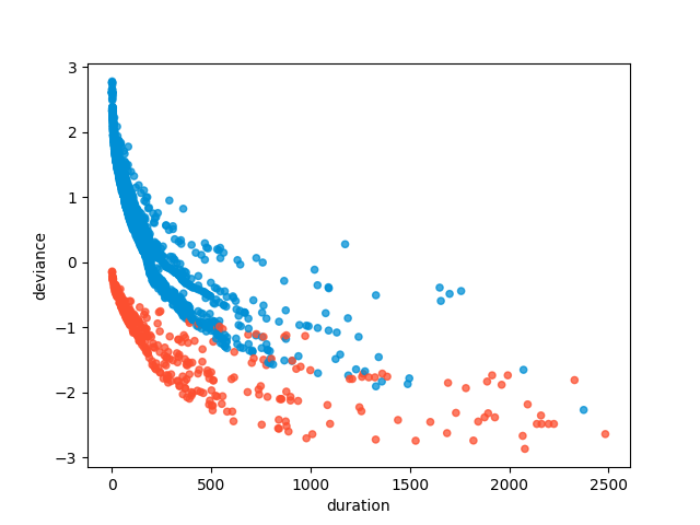
1. When I plot the deviance residuals of the model, a very clear pattern is visible:

(Red dots indicate censored values, blue dots indicate events).

I assume that this pattern indicates that the model is missing some crucial feature which allows it to explain the visible non-linear relation between explanatory and target variable. And it seems to me that the model is underestimating hazard for low durations and overestimating it for large durations (please correct me if I am wrong).

• But why can't the model adapt the hazard function to this slope, as the baseline hazard is non-parametric and thus not bound to any specific distribution of survival times?
• Besides adding other covariables: What could I do to improve the model?

2. Is my interpretation correct that the model says all features except N7460 do have a significant effect on the outcome and that a concordance value of 0.56 tells us that the model does slightly better than plainly guessing average values?

Answer 1

The plots that you show aren't very useful for evaluating a Cox model. Intuition from models like ordinary least squares often doesn't extend to survival modeling.

The baseline hazard over time is necessarily 0 except at observed event times, as the Cox-model hazard is exactly 0 between event times. The lines connecting the points in your first plot are thus, at best, misleading. If you want to show the baseline hazard then show the cumulative hazard, a step function. Remember, however, that the baseline hazard isn't even a part of the Cox model itself. It's something you can extract from the data after you fit the model. It doesn't evaluate the fit of the model.

The discussion of goodness-of-fit measures for survival models in lifelines doesn't include deviance residuals, for good reason. Those coming new to survival modeling often hope to use deviance residuals (or the martingale residuals to which they are related) in the ways that one uses residuals in least-squares modeling. For many purposes you can't, as Therneau and Grambsch explain in Chapter 4. For example, in Section 4.2.3, they note that "martingale residuals and the fitted values are negatively correlated, frequently strongly so," which is related to the plot you show.

With time-fixed covariates, the deviance residuals $d_i$ are close to a normalized difference between the observed $(N_i)$ and predicted $(\hat E_i)$ numbers of events for an individual at the event or censoring time $t_i$ (Therneau and Grambsch, Section 4.3):

$$d_i \approx \frac{N_i(t_i)-\hat E_i(t_i)}{\sqrt {\hat{E_i}(t_i)}}. $$

The numerator is the martingale residual process evaluated at the event or censoring time. The estimated expected number of events for individual $i$ with time-fixed covariate values $X_i$ and corresponding coefficient estimates $\hat \beta$ is a non-decreasing function of time (see Chapter 4 of Therneau and Grambsch):

$$\hat{E_i}(t) = \int_0^t Y_i(s) e^{X_i \hat\beta} d \hat{\Lambda}_0(s),$$

where $Y_i(s)$ is 1 while the individual is at risk (0 otherwise) and $\hat{\Lambda}_0(s)$ is the estimated baseline cumulative hazard over time.

$\hat{E}_i(t)$ is thus related to the estimated baseline cumulative hazard, which has a step increase at each event time over the entire data sample. That has two implications.

First, $\hat{E}_i(t)$ increases by $e^{X_i \hat\beta} d \hat{\Lambda}_0(s)$ at each event time $s$ while at risk. For any set of individuals with the same set of covariate values, the deviance residuals thus necessarily decrease with increasing times to events (or to right censoring).

Second, as the baseline cumulative hazard estimate extends out until the last event in the entire data set, it's quite possible for $\hat{E}_i(t)$ to exceed 1 at a late enough time, if $e^{X_i \hat\beta}$ is large enough.

Put another way, a survival model is of a distribution of event times as a function of covariate values, typically a pretty wide distribution. Some individuals with the same covariate values are going to have event times earlier than "expected" and others will have later event times. That (plus the fact that the deviance residual can't exceed 0 if the event time is censored) is all that your plot of deviance residuals against observation time demonstrates.

Plots of martingale residuals against values of a covariate can be useful to evaluate a model's functional form for a continuous covariate; see this page. What can work more directly than starting from martingale residuals is to use a flexible regression spline to fit a continuous predictor like year_of_manufacture and let the data tell you an approximate functional form.

Finally, the concordance doesn't evaluate "average values" in the way that you seem to think. It's the fraction of pairs of cases for which the observed and model-predicted event orders agree (among case pairs that can be evaluated). It's a measure of discrimination among cases, not calibration. In your case, only 0.56 of pairs had agreement between observed and predicted event orders, close to the 0.5 you would expect by chance.