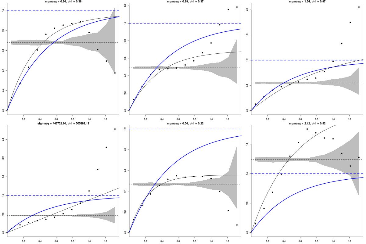
Using grf function from R package geoR, I simulated 6 replicates (each with 1000 samples) of a Gaussian random field on [0, 1] x [0, 1], with zero mean, zero nugget, and an exponential spatial covariance $$\gamma(h) = \exp\left(\frac{h}{\phi}\right)\sigma^2,$$ with $\sigma^2 = 1$ and $\phi = 0.5$. In the following figure, the blue solid curve gives the semi-variogram of this true model and the blue dashed line gives the sill (which is $\sigma^2 = 1$). Then for each replicate, I

1. compute an empirical semi-variogram with function variog (black solid dots);
2. compute a monte-carlo envelope for the empirical semi-variogram (gray shaded polygon);
3. fit an exponential spatial covariance model (black solid curve) to the empirical semi-variogram for $\hat{\sigma}^2$ and $\hat{\phi}$ (printed in the tile).

However, I find it difficult to understand the results / behavior as illustrated by the figure.

1. I simulated data from a true model and fit that true model, why does the fitted semi-variogram differ from the true one so much? Or, why does $(\hat{\sigma}^2, \hat{\phi})$ differ from $(\sigma^2, \phi)$ so much? On some replicate the difference is drastic.
2. How can the empirical semi-variogram (black solid dots), as well as the fitted variogram (black solid curve), breach sample variance (black dashed line)? Isn't sample variance the sill?
3. Why does the black dashed line so much away from the blue dashed line? (the answer is maybe as same as that to question 1)

Is spatial auto-correlation expected to behave like this? If I examine temporal auto-correlation of an AR(1) process by simulating a true time series and fitting it using Yule-Walker methods, I can get back to the truth, i.e., true auto-correlation coefficient and variance. But I can't get this with a spatial process?

Reproducible R code

set.seed(0)

phi <- 0.5
sigmasq <- 1

## unconditional simulation of Gaussian random field with exponential covariance
EXP_GRF <- grf(1000, cov.pars = c(sigmasq, phi), cov.model = "exponential",
               nsim = 6)

## estimation of semi-variogram
semi_variog <- variog(EXP_GRF)

semi_variog_i <- semi_variog
semi_variog_i$v <- NULL

par(mfrow = c(2, 3), mar = c(2.5, 2.5, 1, 1))

for (i in 1:6) {

  ## the i-th empirocal semi-variogram
  semi_variog_i$v <- semi_variog$v[, i]

  ## mc envelops
  env <- variog.mc.env(coords = EXP_GRF$coords, data = EXP_GRF$data[, i],
                       obj.variog = semi_variog_i, nsim = 99, messages = FALSE)

  ## plotting range
  MAX <- max(env$v.lower, env$v.upper, semi_variog_i$v, sigmasq)
  with(semi_variog_i, plot(u, v, ylim = c(0, MAX), type = "n"))

  ## empirical semi-variogram
  polygon(c(semi_variog_i$u, rev(semi_variog_i$u)),
          c(env$v.lower, rev(env$v.upper)), col = 8, border = NA)
  with(semi_variog_i, points(u, v, pch = 19))

  ## variance of the data
  var_data <- semi_variog$var.mark[i]
  abline(h = var_data, lty = 2)

  ## semi-variogram of the true model
  lines.variomodel(EXP_GRF, col = 4, lwd = 2)
  abline(h = sigmasq, lwd = 2, col = 4, lty = 2)

  ## fit an variogram for parameter estimation
  model <- variofit(semi_variog_i, c(var_data, phi), "exponential",
                    fix.nugget = TRUE, nugget = 0, message = FALSE)

  ## fitted variogram
  lines.variomodel(model)

  ## add estimated `sigmasq` and `phi` as title
  title(sprintf("sigmasq = %.2f, phi = %.2f", model[[2]][1], model[[2]][2]))

  }