How to easily obtain the profile likelihood 95% confidence interval for a predicted value in a logistic regression model in R?

Question

I'm a fish biologist and we often use a logistic regression to estimate what we refer to as the L50, i.e. the length at which you expect one fish out of two (50%) to have developed gonads.

How to assess the uncertainty around the L50 estimate is not trivial. Here is an example based on 95 sampled Walleye females that vary in length (LT) from 165 to 680 mm, of which 20 had developed gonads (MATURITE coded as 1) and thus, 75 had undeveloped gonads (MATURITE coded as 0).

The data are referred to as saviMEGI14, and the binary response variable MATURITE is analyzed according to the continuous independent variable LT. The logistic regression model is coded in R like this:

---

summary(m.saviMEGI14.LT <- glm(MATURITE ~ LT, 
   family = binomial, data = saviMEGI14))

---

Using the dose.p() function of the MASS package, I can easily get the estimation of the L50 and its associated SE:

---

library(MASS)

dose.p(m.saviMEGI14.LT)

p = 0.5

Dose = 491.9017

SE = 20.76949

---

And from these estimates, calculate the Wald-based CIs, simply multipling the SE by 1.96 and adding/substracting this value from the "Dose" estimate obtained, i.e. the L50 of 492 mm. The Wald CI would thus be [451, 532].

However, in such a relatively small sample size, the Wald CIs are not ideal because they are based on normal theory, so the default method in R, i.e. the profile likelihood function, should be used instead (see for instance Royston 2007 The Stata Journal)

I am aware that I can get the parameter estimates (central value and CI) for the Intercept and the LT by using the confint() function = profile likelihood or the confint.default() = Wald; but this does not allow me to compute the SE/CIs around the L50 from the logistic regression model.

To get the profile likelihood CIs around the L50 of 492 mm, I use the predict() function applied to the range of LT values by first creating a new data frame called below nd14_LT:

---

nd14_LT <- data.frame(LT=seq(from=165, to=680, 
              by=1))

---

and then get the predicted values for the nd14_LT data, asking also to obtain the associated predicted SE on the logit scale (type="link"):

---

pred14_LT <- predict(m.saviMEGI14.LT, nd14_LT, 
               type="link", se.fit=TRUE)

---

With the predicted values and their associated predicted SE, one can then convert them from the logit to the response scale and then find at which LT a probability of 0.5 is found for both the lower and upper CI bounds.

Doing so provide a profile likelihood-based CI of [457, 551], which is quite different than the Wald one [452, 532], especially for its upper portion.

Here is the plot showing the regression curve, as well as the central value and profile likelihood CIs (which is called a maturity ogive in fisheries science):

All this to come up with this question:

How can someone obtain the lower and upper bounds of the profile likelihood function CI from a logistic regression conducted in R in a rapid manner?

With colleagues, we are using simulations to test different methods for the estimation of the uncertainty around the L50 (i.e., parametric and non-parametric bootstrapping, Fieller analytical method, credible intervals from the Bayesian approach, etc…) and we’d like to find a way to estimate the profile likelihood CI of a given dataset in a timely, valid manner.

Answer 1

My collaborator Rafael de Andrade Moral has written a R function that allows to estimate the uncertainty for L50 estimates according to 13 different methods, including the profile-likelihood method. We used this R function in our recently-published paper in Fisheries Research:

Monitoring reproduction in fish: Assessing the adequacy of ogives and the predicted uncertainty of their L50 estimates for more reliable biological inferences

to evaluate the coverage probability of different approaches, such as the Delta method, non-parametric bootstrapping and Fieller (1944)'s analytical approach. The profile-likehood method did pretty good but the Monte Carlo approach with BCa interval led to the best nominal coverage for the simulated dataset that we have analyzed.

The R scripts for the profile-likelihood method (and others) to assess uncertainty in the L50 (or else such as the L95) is available at:

https://github.com/rafamoral/L50/blob/main/confint_L.R

The supplementary material of our MS contains information on how to use the confint_L() function.

Cheers,

Answer 2

EDIT: I see you mentioned the Fieller method in your original post. Perhaps you were referring to the solution I provided below.

Here is a great paper on the topic. Using a logistic regression with a logit link function you can model the proportion of fish as a function of length, with $\lambda:=$LD50. Based on the asymptotic normality of

$$ \frac{(\hat{\beta}_0 + \lambda\hat{\beta}_1)-\text{ln}\big(\frac{0.5}{1-0.5}\big)}{\sqrt{\hat{\text{se}}_{0}^2 + \lambda^2\hat{\text{se}}_1^2 + 2\lambda\hat{\text{cov}}_{01}}}$$

a $100(1-\alpha)\%$ confidence interval is found by identifying the set of $\lambda$ that satisfy

$$ \frac{\left[(\hat{\beta}_0 + \lambda\hat{\beta}_1)-\text{ln}\big(\frac{0.5}{1-0.5}\big)\right]^2}{\hat{\text{se}}_{0}^2 + \lambda^2\hat{\text{se}}_1^2 + 2\lambda\hat{\text{cov}}_{01}}<z_{\alpha}^2$$

where $\hat{\text{se}}_{0}$ is the estimated standard error of $\hat{\beta}_0$, $\hat{\text{se}}_{1}$ is the estimated standard error of $\hat{\beta}_1$, and $\hat{\text{cov}}_{01}$ is the estimated covariance between $\hat{\beta}_0$ and $\hat{\beta}_1$. This works well even in small sample sizes and is a much better normal approximation than a Wald interval for $\lambda$ based on an identity link using the dose.p() output. The confidence interval above can be calculated using standard output from the logistic regression without calling dose.p(), and should perform similarly to the likelihood ratio CI you are interested in. The only part that would require some work is numerically inverting the quantity above. You can create a sequence of values for $\lambda$, evaluate the quantity above for each value of $\lambda$, and identify those values that satisfy the inequality.

A great way to visualize this is to define and plot the following functions $$H(\lambda)=1-\Phi\Bigg(\frac{(\hat{\beta}_0 + \lambda\hat{\beta}_1)-\text{ln}\big(\frac{0.5}{1-0.5}\big)}{\sqrt{\hat{\text{se}}_{0}^2 + \lambda^2\hat{\text{se}}_1^2 + 2\lambda\hat{\text{cov}}_{01}}}\Bigg)$$

$$H^{\text{-}}(\lambda)=\Phi\Bigg(\frac{(\hat{\beta}_0 + \lambda\hat{\beta}_1)-\text{ln}\big(\frac{0.5}{1-0.5}\big)}{\sqrt{\hat{\text{se}}_{0}^2 + \lambda^2\hat{\text{se}}_1^2 + 2\lambda\hat{\text{cov}}_{01}}}\Bigg)$$

\begin{eqnarray} C(\lambda)= \left\{ \begin{array}{cc} H(\lambda) & \text{if } \lambda\le \hat{\lambda}(\boldsymbol{y}) \\ & \nonumber\\ H^{\text{-}}(\lambda) & \text{if } \lambda\ge \hat{\lambda}(\boldsymbol{y}). \end{array} \right.\nonumber \end{eqnarray}.

where $\hat{\lambda}(\boldsymbol{y})$ is the estimate of LD50 based on the observed data. $C(\lambda)$ is called a confidence curve and depicts p-values and confidence intervals of all levels. In small sample sizes the performance of this interval might be improved by referencing a $t$-distribution with $n-1$ degrees of freedom instead of a standard normal distribution.

If you are still interested in the likelihood ratio test you can create a similar confidence curve:

$$p:=\text{logit}^{-1}({\beta}_0 + \lambda{\beta}_1)$$ $$L(\beta_0,\beta_1)\propto \prod_{i=1}^n \text{logit}^{-1}({\beta}_0 + x_i{\beta}_1)^{y_i}\times[1-\text{logit}^{-1}({\beta}_0 + x_i{\beta}_1)]^{1-y_i}$$ $$\text{LR}=\frac{L(\tilde{\beta}_0,\tilde{\beta}_1)}{L(\hat{\beta}_0,\hat{\beta}_1)}$$ where $\tilde{\beta}_0$ and $\tilde{\beta}_1$ are estimates calculated under the restricted null space for $\lambda$.

\begin{eqnarray} H(\lambda)= \left\{ \begin{array}{cc} \big[1-F_{\chi^2_1}\big(-2\text{log(LR)}\big)\big]/2 & \text{if } \lambda\le \hat{\lambda}(\boldsymbol{y}) \\ & \nonumber\\ \big[1+F_{\chi^2_1}\big(-2\text{log(LR)}\big)\big]/2 & \text{if } \lambda\gt \hat{\lambda}(\boldsymbol{y}). \end{array} \right.\nonumber \end{eqnarray}.

\begin{eqnarray} C(\lambda)= \left\{ \begin{array}{cc} H(\lambda) & \text{if } \lambda\le \hat{\lambda}(\boldsymbol{y}) \\ & \nonumber\\ 1-H(\lambda) & \text{if } \lambda\ge \hat{\lambda}(\boldsymbol{y}). \end{array} \right.\nonumber \end{eqnarray}

where $F_{\chi^2_1}$ is the CDF of a chi-square distribution with 1 degree of freedom. Because the likelihood ratio confidence interval requires profiling nuisance parameters it is almost as computationally intensive as iterative methods such as bootstrap and Monte Carlo approaches.

Answer 3

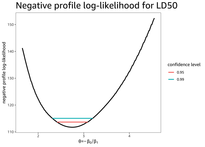
TL;DR @kjetilbhalvorsen explains how to compute confidence intervals based on the profile likelihood in Confidence interval for difference between two predicted probabilities in R. The entire thread is worth reading as it describes several methods to compute confidence intervals. I summarize the profile likelihood method briefly and then apply it to calculate a CI for the median lethal dose, LD50, on the tobacco budworms dataset. See Section 7.2 of Modern Applied Statistics with S by Venables and Ripley.

Let $\theta(\boldsymbol{\beta})$ be a scalar function of the model parameters $\boldsymbol{\beta}$. Then the profile likelihood of $\theta$ is: $$ \begin{aligned} L_P(\theta) = \max_{\theta:\theta(\boldsymbol{\beta})=\theta}L(\boldsymbol{\beta}) \end{aligned} $$ where $L(\boldsymbol{\beta})$ is the likelihood. For the dose-response example, $\boldsymbol{\beta} = (\beta_0,\beta_1)$ but the theory — and the R code — are straightforward to extend to more parameters. The LD50, the dose expected to kill 50% of individuals, is the point where the log-odds of survival are equal to zero: $\theta = -\beta_0/\beta_1$.

x <- budworm$x # dose
y <- budworm$y # survival (0 or 1)

# The LD50 (dose that is expected to kill 50% of individuals) is defined as
# the point where the log-odds of survival are equal to zero.
theta <- function(beta0, beta1) {
  -beta0 / beta1
}

# The negative log-likelihood of the logistic regression model
# with an intercept and one predictor x.
negloglik_lrm <- function(beta0, beta1) {
  prob <- plogis(beta0 + beta1 * x)
  -sum(dbinom(y, 1, prob, log = TRUE))
}

# Fit a simple linear regression to find reasonable starting values.
initialize_betas <- function(x, y) {
  betas <- coef(lm(y ~ x))
  list(beta0 = betas[1], beta1 = betas[2])
}

The crux of the method is to profile the likelihood, ie, to maximize the likelihood over a grid of $\theta$ values. For a fixed $\theta$ we find $\max L(\boldsymbol{\beta})$ over the set $\left\{\boldsymbol{\beta}:\theta(\boldsymbol{\beta})=\theta\right\}$.

# Minimize the negative log-likelihood instead of maximizing the likelihood
model <- bbmle::mle2(negloglik_lrm, start = initialize_betas(x, y))

# nlp = negative profile log-likelihood
grid <- profile_negloglik(model)
grid
#> # A tibble: 201 × 2
#>    theta   npl
#>    <dbl> <dbl>
#>  1  1.65  141.
#>  2  1.67  140.
#>  3  1.68  139.
#>  4  1.70  138.
#>  5  1.71  137.
#>  6  1.73  136.
#>  7  1.74  135.
#>  8  1.75  134.
#>  9  1.77  133.
#> 10  1.78  132.
#> # … with 191 more rows

Now that we have calculated the profile likelihood for $\theta$ at a grid of values, it remains to find a subset of those to represent a confidence interval.

Under regularity conditions (which mean the log likelihood is well approximated by a quadratic function), the ratio likelihood test states that under the null hypothesis $H_0:\theta=\theta_0$: $$ \begin{aligned} 2\log\frac{L(\widehat{\theta})}{L(\theta_0)} \sim \chi^2_p \end{aligned} $$ where $p$ is the number of parameters $\theta$, $\widehat{\theta}$ is the maximum likelihood estimate (MLE) and $\chi^2_p$ is the Chi-squared distribution with $p$ degrees of freedom. This is the value at which the (profile) likelihood is minimized.

By inverting the hypothesis test we get a 100(1-$\theta$)% confidence interval (or region) for $\theta$.

$$ \begin{aligned} \left\{\theta:2\log\frac{L(\widehat{\theta})}{L(\theta)}<\chi^2_{p,(1-\alpha)}\right\} \end{aligned} $$

For the budworms example, the LD50 $\theta$ is a scalar, so $p=1$ and we can find the profile likelihood 95% and 99% confidence intervals numerically:

#>   conf.level conf.low conf.high      nll
#> 1       0.95 2.415057  3.084742 113.6548
#> 2       0.99 2.312052  3.195448 115.0515

I also use the MASS:dose.p function to compute the Wald 95% and 99% confidence intervals. (See R code attached.)

data.frame(
  conf.level,
  conf.low = dose.hat + dose.se * qnorm((1 - conf.level) / 2),
  conf.high = dose.hat - dose.se * qnorm((1 - conf.level) / 2)
)
#>   conf.level conf.low conf.high
#> 1       0.95 2.422786  3.071986
#> 2       0.99 2.320789  3.173983

In this example, the profile and the Wald confidence intervals for $\theta$ agree well.

References

In addition to @kjetilbhalvorsen's posts about profile likelihood, I'm also reading "In All Likelihood: Statistical Modelling And Inference Using Likelihood" by Yudi Pawitan. This book explains the theory in great detail and with many examples. (Not about budworms though.)

---

R code to compute profile likelihood confidence intervals:

library("MASS")
library("tidyverse")

# Compute negative log-likelihood-based intervals for a scalar parameter theta
# at the specified alpha levels.
# This implementation is based on the program `li.r` for computing likelihood
# intervals which accompanies the book "In All Likelihood" by Yudi Pawitan.
# https://www.meb.ki.se/sites/yudpaw/book/
confint_negloglik <- function(theta, nll, conf.level = 0.95) {
  nll_min <- min(nll)
  
  # 2*{ log L(theta_mle) - log L(theta) } < qchisq(df=1,p=1-alpha)
  nll_cut <- nll_min + qchisq(conf.level, 1) / 2
  theta_mle <- mean(theta[nll == nll_min])

  theta_below <- theta[theta < theta_mle]
  if (length(theta_below) < 2) {
    conf.low <- min(theta)
  } else {
    nll.below <- nll[theta < theta_mle]
    conf.low <- approx(nll.below, theta_below, xout = nll_cut)$y
  }

  theta_above <- theta[theta > theta_mle]
  if (length(theta_above) < 2) {
    conf.high <- max(theta)
  } else {
    nll.above <- nll[theta > theta_mle]
    conf.high <- approx(nll.above, theta_above, xout = nll_cut)$y
  }

  data.frame(conf.level, conf.low, conf.high, nll = nll_cut)
}

grid_params <- function(model, pts = 100) {
  seq_range <- function(x, n) {
    seq(min(x), max(x), len = n)
  }
  # Use the confidence intervals to find reasonable ranges for the betas.
  range_betas <- bbmle::confint(bbmle::profile(model))
  expand_grid(
    # Create a grid (= an outer product) for beta0 and beta1
    beta0 = seq_range(range_betas["beta0", ], pts),
    beta1 = seq_range(range_betas["beta1", ], pts)
  ) %>%
    # For each point in the grid, compute the parameter of interest theta
    # and the negative log-likelihood of the model. Both are functions of
    # the regression coefficients beta0 and beta1.
    mutate(
      theta = theta(beta0, beta1),
      nll = map2_dbl(beta0, beta1, negloglik_lrm)
    )
}

profile_negloglik <- function(profile, bins = 201) {
  profile %>%
    grid_params() %>%
    group_by(
      # Subdivide the observed range of theta into many small intervals.
      cut_interval(theta, bins),
      .drop = TRUE
    ) %>%
    summarise(
      # For each interval, find its midpoint as well as the minimum of
      # the negative log-likelihood. This is the negative profile
      # log-likelihood (npl).
      theta = (min(theta) + max(theta)) / 2,
      npl = min(nll)
    ) %>%
    select(
      theta, npl
    )
}

plot_profile <- function(grid, confint) {
  grid %>%
    ggplot(
      aes(theta, npl)
    ) +
    geom_line(
      linewidth = 1
    ) +
    geom_segment(
      aes(
        x = conf.low, xend = conf.high,
        y = nll, yend = nll,
        color = factor(conf.level)
      ),
      inherit.aes = FALSE,
      data = confint,
      linewidth = 1
    ) +
    guides(
      color = guide_legend(title = "confidence level")
    )
}

# Tobacco budworms survival data. See `MASS::dose.p`.
ldose <- rep(0:5, 2)
numdead <- c(1, 4, 9, 13, 18, 20, 0, 2, 6, 10, 12, 16)
numalive <- 20 - numdead

budworm <- list(
  x = c(rep(ldose, numdead), rep(ldose, numalive)),
  y = c(rep(0, sum(numdead)), rep(1, sum(numalive)))
)

conf.level <- c(0.95, 0.99)

x <- budworm$x
y <- budworm$y

# The negative log-likelihood of the logistic regression model
# with an intercept and one predictor x.
negloglik_lrm <- function(beta0, beta1) {
  prob <- plogis(beta0 + beta1 * x)
  -sum(dbinom(y, 1, prob, log = TRUE))
}

# The LD50 (dose that is expected to kill 50% of individuals) is defined as
# the point where the log-odds of survival are equal to zero.
theta <- function(beta0, beta1) {
  -beta0 / beta1
}

# Fit a simple linear regression to find reasonable starting values.
initialize_betas <- function(x, y) {
  betas <- coef(lm(y ~ x))
  list(beta0 = betas[1], beta1 = betas[2])
}

# Minimize the negative log-likelihood instead of maximizing the likelihood
model <- bbmle::mle2(negloglik_lrm, start = initialize_betas(x, y))

profile <- bbmle::profile(model)
grid <- profile_negloglik(model)
grid

# Profile confidence intervals for the betas parameters and for theta
ci.betas <- bbmle::confint(profile)
ci.betas
ci.theta <- confint_negloglik(grid$theta, grid$npl, conf.level)
ci.theta

plt <- plot_profile(grid, ci.theta)
plt +
  labs(
    x = expression(paste(θ, "=", -beta[0] / beta[1])),
    y = "negative profile log-likelihood",
    title = "Negative profile log-likelihood for LD50"
  )

model <- glm(
  y ~ x,
  family = binomial
)

dose.p(model)
dose.hat <- 2.747386
dose.se <- 0.1656153

# Wald confidence interval
data.frame(
  conf.level,
  conf.low = dose.hat + dose.se * qnorm((1 - conf.level) / 2),
  conf.high = dose.hat - dose.se * qnorm((1 - conf.level) / 2)
)