General Question: Should Legitimate Outliers in the Data be Included or Excluded from Statistical Models? [duplicate]

Question

I have the following (general) question (I know there is no definite answer to this question and it largely depends on the specific data and choice of model): Should Legitimate Outliers in the Data be Included or Excluded from Statistical Models?

In general, I have heard both viewpoints argued:

• Include Outliers: I have heard some people argue that outliers should be included in the data because they might contain valuable information about the data that might be able to benefit the statistical model if similar such points are found in the future (e.g. "push" the predicted value of an outlier point away from the mean of all points and closer to the mean value of similar points)

• Exclude Outliers: I have also heard some people argue the opposite - claiming that even if outliers are included in the data used to build statistical models, the "amount" these existing outliers have to "push" the predicted value of "future outliers" closer to themselves is negligible; and on the contrary, including the outliers will jeopardize the predicted values of non-outlier points. In other words, even the most sophisticated models are unable to consistently and accurately predict "black swan events" (i.e. outliers) - and the moment that "black swan events" become somewhat predictable, they paradoxically cease to become "black swan events".

To further explore this issue, I decided to run a small experiment using the R programming language. In this experiment, a random dataset is generated and a small set of random outliers are also generated - a statistical model is first fit to only the random dataset, and a similar statistical model is then fit to the random dataset along with the random outliers. Afterwards, the performance (i.e. error) of both models are evaluated on randomly generated data from similar distributions used to create the intimal dataset, as well as randomly generated data from similar distributions used to create the outliers.

Part 1: Generate Data

#generate data
my_data = data.frame(var_1 = rnorm(100, 10,5), var_2 = rnorm(100,1,1))
my_data$col = as.factor("Non-Outlier")

#generate outliers
outliers = data.frame(var_1 = rnorm(5, 50,5), var_2 = rnorm(5,8,1))
outliers$col = as.factor("Outlier")

#add outliers to data set
my_data_with_outliers = rbind(my_data, outliers)

 head(my_data)


      var_1       var_2         col
1 16.087191 -0.01218058 Non-Outlier
2 14.876278  1.15732819 Non-Outlier
3  7.960061 -0.07095209 Non-Outlier
4  4.136675 -0.59932875 Non-Outlier
5 16.949345  2.60080989 Non-Outlier
6 13.242244  1.81808359 Non-Outlier
    
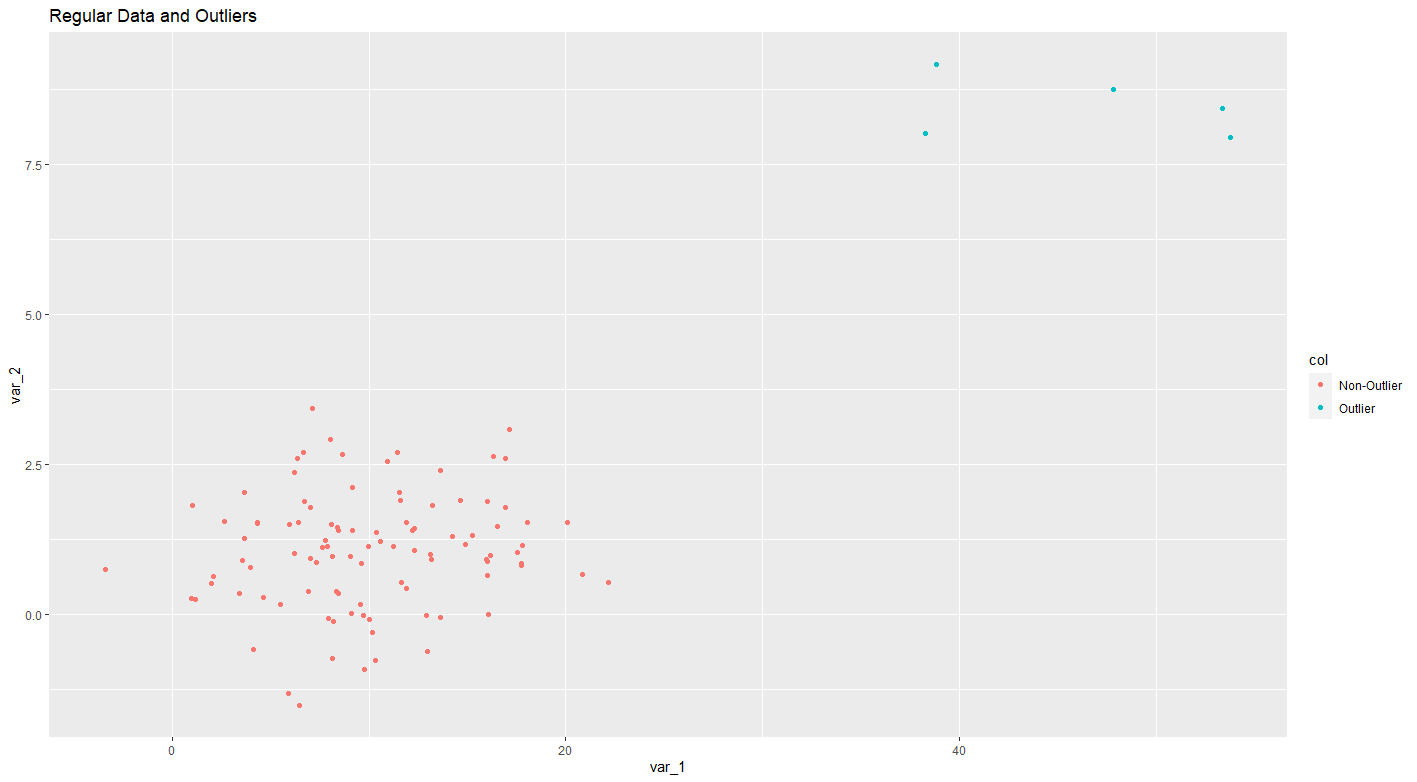
#visualize results

ggplot(my_data_with_outliers, aes(x=var_1, y=var_2, col = col)) +
  geom_point() + ggtitle("Regular Data and Outliers")

Part 2: Statistical Modelling

# Model Without Outliers

model_1 = lm(formula = var_2 ~ var_1, data = my_data)

summary(model_1)


Call:
lm(formula = var_2 ~ var_1, data = my_data)

Residuals:
     Min       1Q   Median       3Q      Max 
-2.49498 -0.60467  0.00899  0.56097  2.43779 

Coefficients:
            Estimate Std. Error t value Pr(>|t|)    
(Intercept)  0.81260    0.21710   3.743 0.000307 ***
var_1        0.02444    0.01938   1.261 0.210136    
---
Signif. codes:  0 ‘***’ 0.001 ‘**’ 0.01 ‘*’ 0.05 ‘.’ 0.1 ‘ ’ 1

Residual standard error: 0.9662 on 98 degrees of freedom
Multiple R-squared:  0.01598,   Adjusted R-squared:  0.005937 
F-statistic: 1.591 on 1 and 98 DF,  p-value: 0.2101

# Model With Outliers

model_2 = lm(formula = var_2 ~ var_1, data = my_data_with_outliers)

summary(model_2)

Call:
lm(formula = var_2 ~ var_1, data = my_data_with_outliers)

Residuals:
    Min      1Q  Median      3Q     Max 
-2.4234 -0.9164  0.0604  0.7067  3.7377 

Coefficients:
            Estimate Std. Error t value Pr(>|t|)    
(Intercept) -0.33647    0.19446   -1.73   0.0866 .  
var_1        0.14848    0.01298   11.44   <2e-16 ***
---
Signif. codes:  0 ‘***’ 0.001 ‘**’ 0.01 ‘*’ 0.05 ‘.’ 0.1 ‘ ’ 1

Residual standard error: 1.233 on 103 degrees of freedom
Multiple R-squared:  0.5595,    Adjusted R-squared:  0.5552 
F-statistic: 130.8 on 1 and 103 DF,  p-value: < 2.2e-16

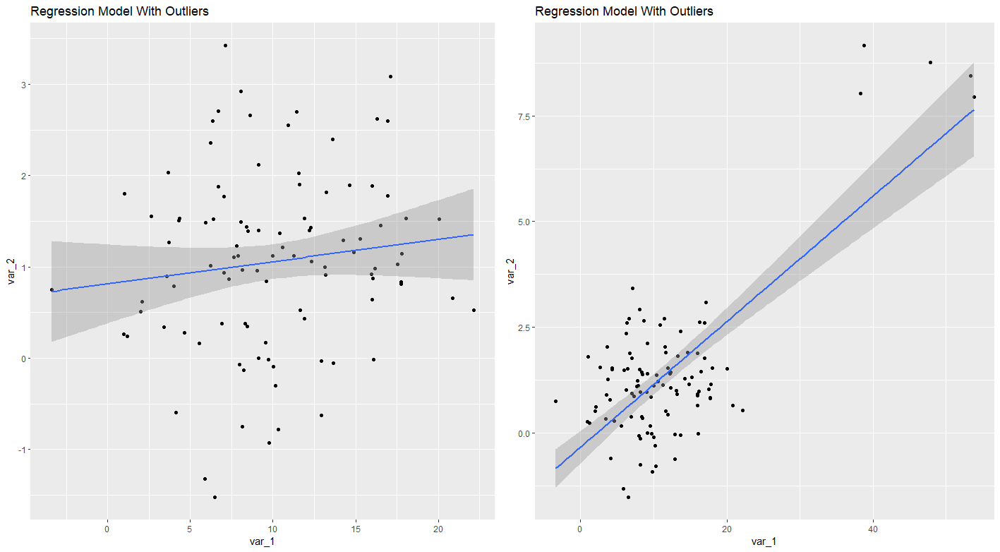
#plot results

ggplot(my_data, aes(x=var_1, y=var_2)) + 
  geom_point()+
  geom_smooth(method=lm) + ggtitle("Regression Model Without Outliers")

ggplot(my_data_with_outliers, aes(x=var_1, y=var_2, col = col)) + 
  geom_point()+
  geom_smooth(method=lm) + ggtitle("Regression Model With Outliers")

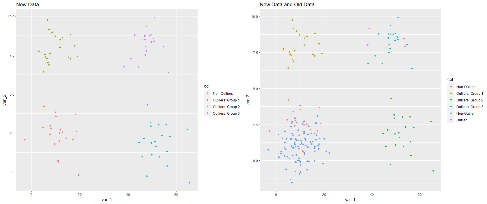
Part 3: Generate 4 Groups of Random Data from the Four Quadrants of the Graph (3 of these are Outliers, 1 of them is not)

#similar to original data
nd1 = data.frame(var_1 = rnorm(20, 10,5), var_2 = rnorm(20,2,1))
nd1$col = as.factor("Non-Outliers")

nd2 = data.frame(var_1 = rnorm(20, 10,5), var_2 = rnorm(20,8,1))
nd2$col = as.factor("Outliers: Group 1")

nd3 = data.frame(var_1 = rnorm(20, 50,5), var_2 = rnorm(20,2,1))
nd3$col = as.factor("Outliers: Group 2")

#similar to initial outliers
nd4 = data.frame(var_1 = rnorm(20, 50,5), var_2 = rnorm(20,8,1))
nd4$col = as.factor("Outliers: Group 3")

new_data = rbind(nd1,nd2, nd3, nd4)

# plot results

ggplot(new_data, aes(x=var_1, y=var_2, col = col)) +
  geom_point() + ggtitle("New Data")

ggplot(rbind(new_data, my_data_with_outliers), aes(x=var_1, y=var_2, col = col)) +
  geom_point() + ggtitle("New Data and Old Data")

Part 4: Error Analysis

outliers = rbind(nd1, nd2, nd3, nd4)

outliers$Model_Without_Outliers_predicted_value =   0.81260  + (0.0244*outliers$var_1)
outliers$Model_With_Outliers_predicted_value =  -0.33647    + ( 0.148  *outliers$var_1)

 outliers$Model_Without_Outliers_error = abs(outliers$Model_Without_Outliers_predicted_value - outliers$var_2)
 outliers$Model_With_Outliers_error = abs(outliers$Model_With_Outliers_predicted_value - outliers$var_2)

head(outliers)
      var_1     var_2                               col Model_Without_Outliers_predicted_value Model_With_Outliers_predicted_value Model_Without_Outliers_error Model_With_Outliers_error
1 11.861975 2.7292896 Outliers (Non-Outliers): Group 1                               1.1020322                           1.4191023                    1.6272574                 1.3101873
2  4.616415 2.8317608 Outliers (Non-Outliers): Group 1                               0.9252405                           0.3467594                    1.9065203                 2.4850014
3 11.658234 1.9678253 Outliers (Non-Outliers): Group 1                               1.0970609                           1.3889486                    0.8707644                 0.5788767
4 10.091540 3.5421764 Outliers (Non-Outliers): Group 1                               1.0588336                           1.1570779                    2.4833428                 2.3850985
5 11.173635 0.6196431 Outliers (Non-Outliers): Group 1                               1.0852367                           1.3172279                    0.4655936                 0.6975849
6 -2.916149 2.0538053 Outliers (Non-Outliers): Group 1                               0.7414460                          -0.7680600                    1.3123594                 2.8218654

#summarize results

library(dplyr)
library(gt)
    
#use median residuals from both models for "row 5"

gt(outliers %>%
    group_by(col) %>%
    dplyr::summarize(Mean_Prediction_Error_Model_Without_Outliers = mean(Model_Without_Outliers_predicted_value, na.rm=TRUE), Mean_Prediction_Error_Model_With_Outliers = mean(Model_With_Outliers_predicted_value, na.rm=TRUE))  %>% add_row(col = "Original Data", Mean_Prediction_Error_Model_Without_Outliers = 0.008,  Mean_Prediction_Error_Model_With_Outliers = 0.06))

# A tibble: 5 x 3
  col                                 Mean_Prediction_Error_Model_Without_Outliers Mean_Prediction_Error_Model_With_Outliers
  <chr>                                                                      <dbl>                                     <dbl>
1 "Outliers (Non-Outliers): Group 1 "                                        1.08                                       1.27
2 "Outliers: Group 1"                                                        1.06                                       1.14
3 "Outliers: Group 2"                                                        2.09                                       7.42
4 "Outliers: Group 3"                                                        1.98                                       6.73
5 "Original Data"                                                            0.008                                      0.06

My Question: Based on this very specific example of data and choice of model - it seems that the statistical model created using data with the outliers removed, performed better than the statistical model created using the data with the outliers. However, this is a specific example of data and models - there exists an infinite universe of models and data with the opposite outcome (i.e. the model created with outliers performs better than the model without outliers) can be equally as likely.

In general - are outliers often identified, excluded from the statistical model and studied for the purpose of better understanding the data; or are the outliers often left in the data and used to push the predicted value of future outlier points away from the sample mean?

Can someone please comment on this? Would anyone like to share any anecdotes or personal experiences regarding this topic? Are there any statistical models (e.g. decision trees, random forest, kernel based models, neural networks) which are more/less sensitive to outliers? Do outliers pose more of a problem in some types of problems compared to others (e.g. classification vs. regression)?

Thanks!

Note: If outliers can be identified as "not legitimate" (e.g. negative human height, human age over 130 years, etc. - from data entry errors, data corruption, misreported data, etc.) , it would more sense that these outliers be removed.

Answer 1

I will answer this question in theoretical perspective.

I think you should include legitimate outliers in your statistical model. I want to share my one experience with you for my undergrad project I was building a machine learning model that could predict revenue of a private bank and transaction density at first, I intentionally removed all the outliers from my statistical modelling. But when we tried to run the model on real time data of the bank after some months the model was underperforming then second wave of COVID came and the transaction became very less than normal. So, our model gets out of the production as it couldn't understand what was going on.

My professor said we can easily predict upcoming revenue using statistics but what a ML model should do is to predict anomaly in the system which is coming for this, we need some outliers to prepare our model for whatever hard situation ahead.

What I am trying to say including outliers at some degree can really help your model to be robust and handle some hard truth.