Time Series Forecasting With "Seasonal Gaps"?

Question

Suppose I have the following problem - we are interested in modelling the number of animals that cross a certain point each year (e.g. swim across a river). Let's say that these animals typically migrate during the summer months (e.g. April - September), and in the winter months this number becomes almost becomes 0.

Suppose I have 10 years of data collected at the weekly level - this means that in the winter months, the number of animals that cross this point are basically 0. Thus, there are large natural "gaps" that occur within the data.

When such situations arise, is it generally better to fit a time series model (e.g. ARIMA) to the entire dataset and treat each year as a cycle - or is it better to construct cycles out of the "active months" that contain data?

E.g.

• Option 1 - Stack Rows from Each Subset on Top of Each Other to Create a Modified Dataset: (April 2010 - September 2010, April 2011 - September 2011, April 2012 - September 2012,etc.)
• Option 2 - Simply Model the Entire Dataset: April 2010 - April 2020

In general, is it better to fit time series models to datasets created from Option 1 or Option 2? Are some models (e.g. arima, ets, regime switch models) more suitable for this kind of problems(e.g. some models perhaps might make negative predictions or negative confidence intervals when the response variable is low)?

Answer 1

I would model the data generating process using the entire dataset. From what you described I believe you are dealing with a Zero-Inflated count process. We can model such a process using a zero-inflated Poisson model. A simple form of such model can be written as:

\begin{align} y_{t} &\sim \text{Poisson}(\lambda_{t}) \\ \end{align}

\begin{align} \lambda_{t} = \mu_{week[t]} \times x_{t}\\ \end{align}

\begin{align} x_{t} &\sim \text{Bernoulli}(p_{t}) \\ \end{align}

\begin{align} logit(p_{t}) &= \theta_{week[t]} \end{align}

Here I am assuming that the only predictor is the week of the year (each week has its own effect). Since you have not provided your data, I simulate some data myself and fit the model using JAGS in R. The code is as follows:

library(R2jags)
library(tidyverse)

n <- 52 * 10 #Total num of observations: 52 weeks x 10 years
set.seed(123)

df <- data.frame(time = seq(1,n,1),
                 year = rep(2010:2019, each = 52),
                 week = rep(1:52, 10)) %>% 
        mutate(observed = rpois(nrow(.), 10),
               observed = ifelse(week >= 49 | week <= 14, 0, observed)) # set observed counts to zero during winter

As you can see, I set the observed counts during winter to zero. But for other times the counts follow a Poisson distribution with mean 10. I fit the model using JAGS in R as follows:

# ---- JAGS model ----
mod_string = "model {
  for (i in 1:length(y)) {
    # Likelihood
    y[i] ~ dpois(lambda[i])

    # Linear predictor
    lambda[i] <- mu[week[i]]*x[i] + 0.00001 # (0.00001: hack required for Rjags)
    
    # Zeros model
    x[i] ~ dbern(pro[i])
    logit(pro[i]) <- theta[week[i]]
    
  }
  # Priors
  for (w in 1:52){
  
    theta[w] ~ dnorm(0, 1^-2)
    mu[w] ~ dnorm(0, 10^-2)
    
    }
}"

# ---- Data ----
data_jags = list(y = df$observed, 
             week = df$week)

# ---- Parameters to save ----
params = c('theta', 'mu', 'lambda')


# ---- Run the model ----
model_run <- jags(
  data = data_jags,
  parameters.to.save = params,
  model.file = textConnection(mod_string)
)

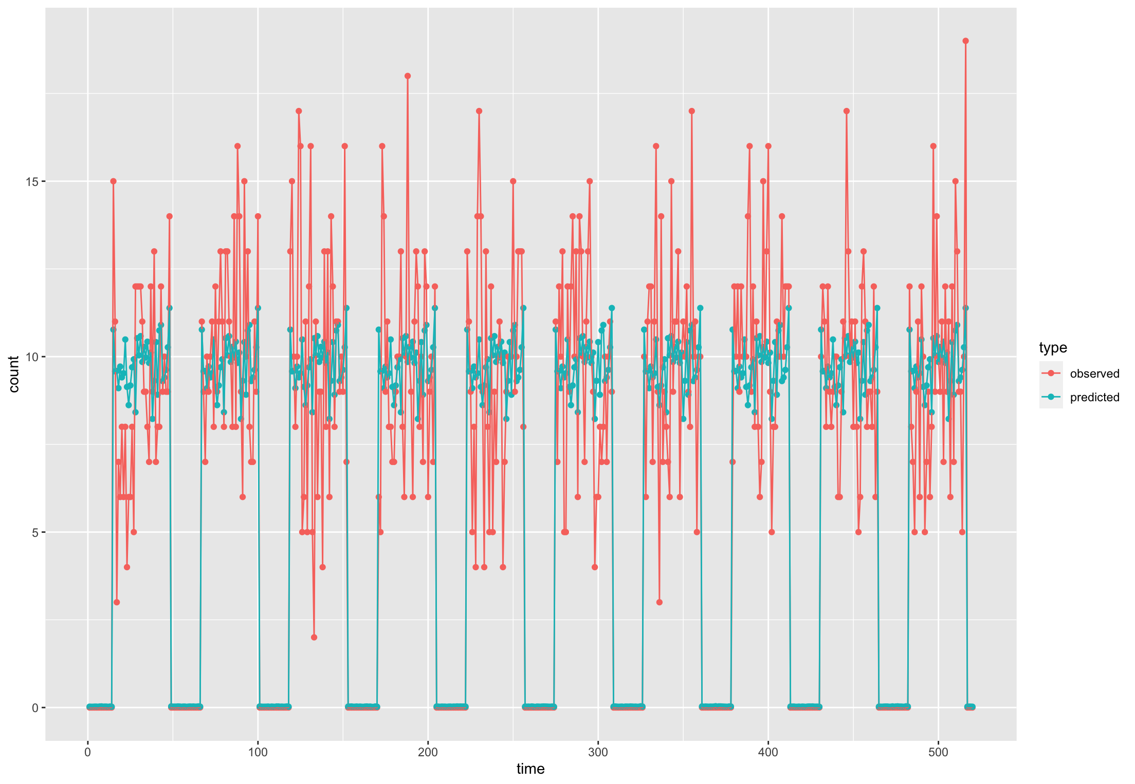
We can extract the posterior samples from the model and plot the model output against the observed data like below:

# ---- Extract posterior mean ----
df$predicted <- model_run$BUGSoutput$mean$lambda 

# ---- Plot observed versus posterior means over time ----
df %>% 
  pivot_longer(names_to = 'type', values_to = 'count', -c(time:week)) %>% 
  ggplot(aes(time, count, color = type)) + geom_point() + geom_line()

This is the results:

Of course you can extend the model and add more covariates or change the structure and add auto regressive components and etc. But I hope this example helps.

Answer 2

I would encourage you to try Option 1 as it's simpler.

It seems that you are most interested in what is happening during the busy months of April-September, and I imagine are probably interested in the form the model takes (e.g. if you fit an AR(1) model you may be very interested in the value the AR coefficient takes). The issue with including October-March observations is the data generating process is likely quite different, and even if you properly transform your data to correct for constant variance in the errors, it could still impact your model fit for the part of the data you actually care about. For example if April-September was AR(1) with AR coefficient $\phi=0.5$ and October-March was AR(1) with $\phi=-0.5$, then the fitted model would end up with $\phi\approx0$, which may lead you to make incorrect inferences about the data generating process during the busy months.

When fitting the model you probably want to try two ways of dealing with the gaps. In the case of the AR(1) model you could try either of

$$\begin{align}X_{\text{April2021}}&=\phi X_{\text{March2021}}+\epsilon_{\text{April2021}}\\ X_{\text{April2021}}&=\phi X_{\text{September2020}}+\epsilon_{\text{April2021}} \end{align}$$ and see what looks best. Also you can modify the equations accordingly if you want to incorporate seasonality.