Can I use 'mean ± SD' for non-negative data when SD is higher than mean? [duplicate]

Question

This time, I calculated a non-negative dataset which SD is larger than mean

I have seen many people use 'mean ± SD' to show mean and standard deviation.

But I wonder whether we can use that form for non-negative dataset.

The original data can't be lower than 0 but if I use ± it looks can be negative number(like 1 ± 3).

Is their no problem or should I use other way?

Answer 1

[edited based on helpful feedback in the comments]

It bothers me immensely when people do this. The argument against it is simple: the standard deviation is typically shown to convey information about data distribution (and standard error for a parameter). It achieves this goal well in some situations but not others. If the standard deviation/error implies that negative values are reasonable when you know they are not, it is not helping you communicate accurately. Bimodal distributions are another situation in which mean ± SD/SE is likely to mislead.

So what else can you do? If you're interested in the data distribution, just show the full distributions using density plots, violin plots, histograms, or their alternatives. If you're interested in the uncertainty of a parameter, you could show confidence intervals or the posterior distribution. Unlike standard deviation or standard error, these options can be asymmetric and will communicate the data distribution or uncertainty more accurately.

If you must use a numerical summary for a data distribution without referring to a graph, you could use quartiles instead of mean ± SD.

Answer 2

'Mean ± SD' is notation. Once you define it in a manner visible to the reader, you can use it in that manner regardless of the values.

When your statistics are skewed enough that they are positive with a standard deviation larger than the mean, the question is whether describing them in terms of mean and standard deviation is really sensible because cumulants other than mean and variance will be highly relevant for the distribution, making it significantly different from a normal distribution (for which mean and variance are the only non-zero cumulants).

Chances are that the logarithm of your positive random variable is quite better approaching a normal distribution and parameterising that makes more sense.

Answer 3

In cases like yours, I've reported the median and the quartiles, as mkt suggested.

But, inspired by the OverLordGoldDragon's answer and motivated by the wish to keep the idea of the mean and sd and, at the same time, not to deviate too much from established statistical practices, I propose an alternative. I don't know whether it's been used so far, so I'll call it the "decomposed standard deviation". It also allows you to report the results as three numbers, in the form $\overline x ~ (+sd_A; -sd_B)$.

Standard deviation is: $$ sd = \sqrt{\frac{1}{N-1}\sum_i (x_i - \overline x)^2}. $$ The sum can be decomposed into the sum over the elements above and below $\overline x$: $$ sd = \sqrt{\frac{1}{N-1} \left( \sum_{i:x_i \gt \overline x} (x_i - \overline x)^2 + \sum_{i:x_i < \overline x} (x_i - \overline x)^2 \right)} $$

(I've left out the summation over $i: x_i = \overline x$, as it evaluates to zero).

Define: $$ \begin{align} sd_A &= \sqrt{\frac{1}{N_A + \frac{N_0-1}{2}} \sum_{i:x_i \gt \overline x} (x_i - \overline x)^2 }, \\ sd_B &= \sqrt{\frac{1}{N_B + \frac{N_0-1}{2}} \sum_{i:x_i \lt \overline x} (x_i - \overline x)^2 } \end{align} $$ with $N_A$, $N_B$, and $N_0$ being the number of elements "above", "below" and "equal to" the mean, respectively. Then, the standard deviation can be rewritten as: $$ sd = \sqrt{\frac{(N_A + \frac{N_0-1}{2})sd_A^2 + (N_B + \frac{N_0-1}{2})sd_B^2} {N-1} }. $$ If no values are exactly equal to $\overline x$, which is very likely in practice, the formulae simplify to: $$ \begin{align} sd_A &= \sqrt{\frac{1}{N_A - 0.5} \sum_{i:x_i \gt \overline x} (x_i - \overline x)^2 }, \\ sd_B &= \sqrt{\frac{1}{N_B - 0.5} \sum_{i:x_i \lt \overline x} (x_i - \overline x)^2 }, \\ sd &= \sqrt{\frac{(N_A -0.5)sd_A^2 + (N_B - 0.5)sd_B^2} {N-1} }. \end{align} $$

It is easy to show that for perfectly symmetric data, $sd$, $sd_A$, and $sd_B$ are exactly the same. For asymmetric, they differ. Also, it is easy to see that for non-negative data, $\overline x - sd_B$ is always non-negative.

Below is a simple graphical example:

and you'd report the result as $1.56 ~ (+3.08; -0.93)$. This makes the asymmetry in the data explicit and, at the same time, avoids the implication that data can be negative.

Below is the Python code to reproduce the figure and play with the data:

import matplotlib.pyplot as plt
import numpy as np


def decomposed_std(x):
  m = x.mean()  
  xA = x[x > m]
  xB = x[x < m]
  nA = len(xA)
  nB = len(xB)
  n0 = len(x[x == m])
  sA = np.sqrt(np.sum((xA-m)**2) / (nA + (n0-1)/2))
  sB = np.sqrt(np.sum((xB-m)**2) / (nB + (n0-1)/2))
  # the two are equal:
  # np.sqrt((sA**2 * (nA + (n0-1)/2) + sB**2 * (nB + (n0-1)/2)) / (n-1))
  # x.std(ddof=1)
  return sA, sB
  

np.random.seed(0)
x = np.exp(np.random.normal(0, 1, 1000))
m = x.mean()
x = np.hstack([x, [m, m, m, m, m]]) # append some averages

s = x.std(ddof=1)
sA, sB = decomposed_std(x)

h = plt.hist(x, bins=20, fc='skyblue', ec='steelblue')
y_top = max(h[0])
x_right = max(h[1])
plt.vlines(x.mean(), 0, 1.1*y_top, colors='chocolate')
plt.plot([m-sB, m], [1.025*y_top]*2, '-', color='seagreen')
plt.plot([m+sA, m], [1.025*y_top]*2, '-', color='firebrick')
plt.grid(linestyle=':')
plt.text(0.8*m, 1.05*y_top, f'$sd_B = {sB:.2f}$', horizontalalignment='right')
plt.text(1.2*m, 1.05*y_top, f'$sd_A = {sA:.2f}$', horizontalalignment='left')
plt.text(x_right, 1.1*y_top,
          '$\overline{x} = ' f'{m:.2f}$\n'
          '$sd = ' f'{s:.2f}$',
          horizontalalignment='right', verticalalignment='top')
plt.title('Histogram with decomposed standard deviation')
plt.xlim(-2, 1.05*x_right)
plt.show()

Answer 4

You use mean ± SD to summarize the distribution of your data and mean ± SE to indicate the uncertainty of your estimate of the mean. However, mean ± SD might provide a bad summary of the distribution, as seems to be the case for your data. Then you must look around for other descriptors to provide the shorthand summary. If space is not an issue, show the distribution with a histogram, density plot or whatever. It might be worth the effort to identify the distribution of your data (negative binomial, Poisson, or whatever) and provide the distribution parameters as a summary.

Answer 5

Sometimes for positive data it can make sense to report the mean and standard deviation of the log of the data rather than the data itself. This is arguably the best summary you can give if the data seems to follow an approximately log-normal distribution. The answer to this question probably gives a better discussion of this option than I can.

Answer 6

If your intention is to summarize the spread of your data, then just standard deviation, variance, range or coefficient of variation can be sufficient. In your case, you should compute modes to check whether your data follows a multimodal distribution as well. However I cannot see any reason just differencing standard deviation from the mean would inform you about the dataset. I would use median, mode and range values to summarize that dataset.

This operation is probably inspired by the construction of confidence intervals for the estimation of a population mean. However, these intervals are constructed randomly and utilizes information about the distribution of the random variable in question to infer how likely the true population parameter is in many intervals calculated in the same manner. In essence, it tests how stable your estimation is concerning the mean. That is often done to support hypothesis tests for population parameters. I see distribution information is completely discarded here, which may be the reason that you obtain irrelevant, negative values.

Edit: I also cannot see any reason to prefer "standard deviations above and below the mean", as some answers have suggested, over computing first and third quartiles or interquartile range (in general, L-estimators); then again, if your goal is to inform about the spread in your data.

Answer 7

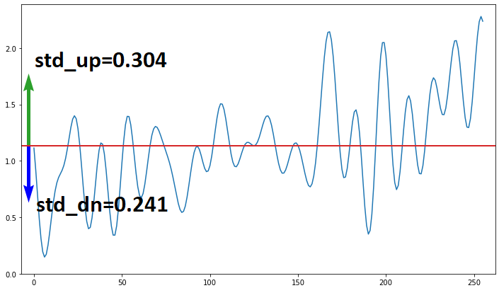
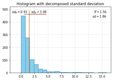
It varies with context, I present one option - "directional standard deviation": compute SD separately above and below mean:

If the goal is a measure of spread of data, this can work.

Arithmetic mean isn't always best - could try median, another averaging metric, or for sparse data, "sparse mean" that I developed and applied on an audio task.

std = lambda x, x_mean: np.sqrt(1 / len(x) * np.sum((x - x_mean)**2))
x_mean = x.mean()
std_up = std(x[x >= x_mean], x_mean)
std_dn = std(x[x <  x_mean], x_mean)

This was typed in a hurry and isn't polished; no consideration was given to handling x == x.mean() for equivalence with usual SD via constant rescaling, or to whether < should be <=, but it can be done, refer to @IgorF.'s answer.

Clarification

This is simply feature engineering. It has nothing to do with statistical analysis or describing a distribution. SD (standard deviation) is a nonlinear alternative to mean absolute deviation with a quadratic emphasis.

I saw a paper compute SD from 3 samples. I first-authored it and remarked it as ludicrous. Then I figure, it just functions as a spread measure, where another metric wouldn't be much better.

Whether there's better ways to handle asymmetry is a separate topic. Sometimes SD is best for similar reasons it's normally best. I can imagine it being a thresholding feature in skewed non-negative data.

Connection to question

I read the question, going off of the title and most of the body, as: "I want to use SD but want to stay non-negative". Hence, a premise is, SD is desired - making any objections to SD itself irrelevant. Of course, the question can also read as "alternatives to SD" (as it does in last sentence), but I did say, "I present one option".

More generally, any objections to my metric also hold for SD itself. There's one exception, but often it's an advantage rather than disadvantage: each number in my metric has less confidence per being derived from less data. This can be advantage since, it's more points per sub-distribution. Imagine,

SDD = "standard deviation, directional". For the right-most example, points to right of mean are only a detriment to describing points to left, and the mismatch in distributions can be much worse than shown here (though it does assume "mean" is the right anchor, hence importance of choosing it right).

Formalizing

@IgorF's answer shows exactly what I intended, minus handling of x == x.mean() which I've not considered at the time, and I favor 1/N over 1/(N-1); I build this section off of that. What I dislike about that mean handling is

[-2, -1, -1, 0,     1, 1, 2] --> (1.31, 1.31), 1.31
[-2, -1, -1, 1e-15, 1, 1, 2] --> (1.41, 1.31), 1.31

showing --> SDD, SD. i.e. the sequences barely differ, yet their results differ significantly - that's an instability. SD itself has other such weaknesses, and it's fair to call this one a weakness of SDD; generally, caution is due with mean-based metrics.

If the relative spread of the two sub-distributions is desired, I propose an alternative:

1. Replace $\geq$ and $\leq$ with $\gtrapprox$ and $\lessapprox$, as in "points within mean that won't change the pre-normalized SD much", "pre-normalized" meaning without square root and constant rescaling.
2. Do this for each side separately.
3. Don't double-count - instead, points which qualify both for > mean and ~ mean are counted toward ~ mean alone, and halve the rescaling contribution of the ~ mean points (as in @IgorF.'s). This assures SDD = SD for symmetric distributions.
4. "won't change much" becomes a heuristic, and there's many ways to do it - I simply go with abs(x - mean)**2 < current_sd / 50

[-2, -1, -1, 0,     1, 1, 2] --> (1.31, 1.31), 1.31
[-2, -1, -1, 1e-15, 1, 1, 2] --> (1.31, 1.31), 1.31

[-2, -1, -1, 3e-1,  1, 1, 2] --> (1.35, 1.29), 1.31
[-2, -1, -1, 5e-1,  1, 1, 2] --> (1.48, 1.19), 1.32

It can be made ideal in sense that we can include points based on not changing sd_up or sd_dn by some percentage, guaranteeing stability, but I've not explored how to do so compute-efficiently.

I've not checked that this satisfies various SD properties exactly, so take with a grain of salt.

Code

import numpy as np

def std_d(x, mean_fn=np.mean, div=50):
    # initial estimate
    mu = mean_fn(x)
    idxs0 = np.where(x < mu)[0]
    idxs1 = np.where(x > mu)[0]
    sA = np.sum((x[idxs0] - mu)**2)
    sB = np.sum((x[idxs1] - mu)**2)

    # account for points near mean
    idxs0n = np.where(abs(x - mu)**2 < sA/div)[0]
    idxs1n = np.where(abs(x - mu)**2 < sB/div)[0]
    nmatch0 = sum(1 for b in idxs0n for a in idxs0 if a == b)
    nmatch1 = sum(1 for b in idxs1n for a in idxs1 if a == b)
    NA = len(idxs0) - nmatch0
    NB = len(idxs1) - nmatch1
    N0A = len(idxs0n)
    N0B = len(idxs1n)
    sA += np.sum((x[idxs0n] - mu)**2)
    sB += np.sum((x[idxs1n] - mu)**2)

    # finalize
    kA = 1 / (NA + N0A/2)
    kB = 1 / (NB + N0B/2)
    sdA = np.sqrt(kA * sA)
    sdB = np.sqrt(kB * sB)
    return sdA, sdB


x_all = [
    [-2, -1, -1, 0,     1, 1, 2],
    [-2, -1, -1, 1e-15, 1, 1, 2],
    [-2, -1, -1, 3e-1,  1, 1, 2],
    [-2, -1, -1, 5e-1,  1, 1, 2],
]
x_all = [np.array(x) for x in x_all]

for x in x_all:
    print(std_d(x), x.std())