Is it possible to apply a monotonicity constraint on a Gaussian process regression fit?

Question

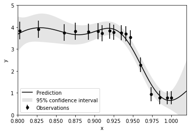
Below is a code using scikit-learn where I simply apply Gaussian process regression (GPR) on a set of observed data to produce an expected fit. I know physically that this curve should be monotonically decreasing, yet it is apparent that this is not strictly satisfied by my fit. I have observed instances where people apply various constraints on GPR (e.g. zero slope at certain x), although is it possible to constraint GPR to produce a monotonically decreasing fit? Are there any kernels in scikit-learn (or custom kernels) that could permit sharp gradients, as displayed around x = 0.95, while still favouring monotonicity?

import numpy as np
from matplotlib import pyplot as plt
from sklearn.gaussian_process import GaussianProcessRegressor
from sklearn.gaussian_process.kernels import RBF, ConstantKernel as C

def f(x):
    """The function to predict."""
    return 1.5*(1. - np.tanh(100.*(x-0.96))) + 1.5*x*(x-0.95) + 0.4 + 1.5*(1.-x)* np.random.random(x.shape)

# Instantiate a Gaussian Process model
kernel = C(10.0, (1e-5, 1e5)) * RBF(10.0, (1e-5, 1e5))

X = np.array([0.803,0.827,0.861,0.875,0.892,0.905,
                0.91,0.92,0.925,0.935,0.941,0.947,0.96,
                0.974,0.985,0.995,1.0])
X = np.atleast_2d(X).T

# Observations and noise
y = f(X).ravel() 
noise = np.linspace(0.4,0.3,len(X))
y += noise

# Instantiate a Gaussian Process model
gp = GaussianProcessRegressor(kernel=kernel, alpha=noise ** 2,
                              n_restarts_optimizer=10)
# Fit to data using Maximum Likelihood Estimation of the parameters
gp.fit(X, y)

# Make the prediction on the meshed x-axis (ask for MSE as well)
x = np.atleast_2d(np.linspace(0.8, 1.02, 1000)).T
y_pred, sigma = gp.predict(x, return_std=True)

plt.figure() 
plt.errorbar(X.ravel(), y, noise, fmt='k.', markersize=10, label=u'Observations')
plt.plot(x, y_pred, 'k-', label=u'Prediction')
plt.fill(np.concatenate([x, x[::-1]]),
         np.concatenate([y_pred - 1.9600 * sigma,
                        (y_pred + 1.9600 * sigma)[::-1]]),
         alpha=.1, fc='k', ec='None', label='95% confidence interval')
plt.xlabel('x')
plt.ylabel('y')
plt.xlim(0.8, 1.02)
plt.ylim(0, 5)
plt.legend(loc='lower left')
plt.show()

I believe this should be possible as described here by applying virtual inputs, and possibly other elegant methods, although I am just struggling with an actual simple implementation that can be applied to the above code.

Answer 1

The answer is no - you can not exactly enforce monotonic constraints in GPs, but there are a number of approximations which you could make. I believe the most popular (I haven’t read the paper you linked but would assume it also works as follows) is to model the square root or log of the derivative of the function space with a Gaussian process using pseudo points. Another approach is to try to model the derivative with a non-zero mean GP. This won’t be strictly monotonic, but at any point the probability of the function having a negative(or positive) slope is small.

The main problem is that the conditional of a Gaussian process is always a Gaussian and thus there will always be probability mass in the positive and negative side of the previously observed point. So what is a monotonic function? One which has a strictly positive or negative derivative. The derivative of a Gaussian process is also a Gaussian process provides the kernel is differentiable. So modeling the derivative alone will not strictly enforce monotonicity. This is why modeling a strictly positive or negative function of the space with a GP is really the way you might want to go.

However, now you face the next hurdle. The derivative tells only the change in y values between observations. So you don’t really have the right data to do the modeling. You can get around this by modeling the space with pseudo points and using (for example) WASABI GP which allows you to infer quadrature samples from GPs in Square root space - check out Gunter et al. For more on this.

Finally, you might be far better off using another space such as Bernstein polynomials which allows you to perform strictly monotonic polynomial regression.

Answer 2

Just a quick thought: consider the GP $f(t) \sim GP(0, k(t, t'))$ where $k(t,t') = t t'$. This GP is degenerate, which allows it to generate monotonically increasing or decreasing samples. See also Why functions sampled from a linear kernel Gaussian Process are guaranteed to be a linear function?.