Great question! Let's step back and understand what Bonferroni did, and why it was necessary for Benjamini and Hochberg to develop an alternative.
It has become necessary and compulsory in recent years to perform a procedure called multiple testing correction. This is due to the increasing numbers of tests being performed simultaneously with high throughput sciences, especially in genetics with the advent of whole genome association studies (GWAS). Excuse my reference to genetics, as it is my area of work. If we are performing 1,000,000 tests simultaneously at $P = 0.05$, we would expect $50,000$ false positives. This is ludicrously large, and thus we must control the level at which significance is assessed. The bonferroni correction, that is, dividing the acceptance threshold (0.05) by the number of independent tests $(0.05/M)$ corrects for the family wise error rate ($FWER$).
This is true because the FWER is related to test-wise error rate ($TWER$) by the equation $FWER = 1 - (1 - TWER)^M$. That is, 100 percent minus 1 subtract the test wise error rate raised to the power of the number of independent tests performed. Making the assumption that $(1- 0.05)^{1/M} = 1-\frac{0.05}{M}$ gives $TWER \approx \frac{0.05}{M}$, which is the acceptance P value adjusted for M completely independent tests.
The problem that we encounter now, as did Benjamini and Hochberg, is that not all tests are completely independant. Thus, the Bonferroni correction, though robust and flexible, is an overcorrection. Consider the case in genetics where two genes are linked in a case called linkage disequilibrium; that is, when one gene has a mutation, another is more likely to be expressed. These are obviously not independent tests, though in the bonferroni correction they are assumed to be. It is here where we start to see that dividing the P value by M is creating a threshold that is artificially low because of assumed independent tests which really influence each other, ergo creating an M that is too large for our real situation, where things aren't independent.
The procedure suggested by Benjamini and Hochberg, and augmented by Yekutieli (and many others) is more liberal than Bonferroni, and in fact Bonferroni correction is only used in the very largest of studies now. This is because, in FDR, we assume some interdependence on the part of the tests and thus an M which is too large and unrealistic and getting rid of results that we, in reality, care about. Therefore in the case of 1000 tests which are not independent, the true M would not be 1000, but something smaller because of dependencies. Thus when we divide 0.05 by 1000, the threshold is too strict and avoids some tests which may be of interest.
I'm not sure if you care about the mechanics behind the controlling for dependency, though if you do I have linked the Yekutieli paper for your reference. I'll also attach a few other things for your information and curiosity.
Hope this has helped in some way, if I have misrepresented anything please do let me know.
~ ~ ~
References
Yekutieli paper on positive dependencies -- http://www.math.tau.ac.il/~ybenja/MyPapers/benjamini_yekutieli_ANNSTAT2001.pdf
( see 1.3 -- The Problem. )
Explaination of Bonferroni and other things of interest -- Nature Genetics reviews. Statistical Power and significance testing in large-scale genetic studies -- Pak C Sham and Shaun M Purcell
( see box 3. )
http://en.wikipedia.org/wiki/Familywise_error_rate
EDIT:
In my previous answer I did not directly define positive dependency, which was what was asked. In the Yekutieli paper, section 2.2 is entitled Positive dependence, and I suggest this as it is very detailed. However, I believe that we can make it a little bit more succinct.
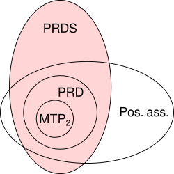
The paper at first begins by talking about positive dependancy, using it as a vague term that is interpretable but not specific. If you read the proofs, the thing that is mentioned as positive dependency is called PRSD, defined earlier as "Positive regression dependancy on each one from a subset $I_0$". $I_0$ is the subset of tests that correctly support the null hypothesis (0). PRDS is then defined as the following.

$X$ is our whole set of test statistics, and $I_0$ is our set of test statistics which correctly support the null. Thus, for $X$ to be PRDS (positively dependent) on $I_0$, the probability of $X$ being an element of $I_0$ (nulls) increases in non decreasing set of test statistics $x$ (elements of $X$).
Interpreting this, as we order our $P$-values from lowest to highest, the probability of being part of the null set of test statistics is the lowest at the smallest P value, and increases from there. The FDR sets a boundary on this list of test statistics such that the probability of being part of the null set is 0.05. This is what we are doing when controlling for FDR.
In summation, the property of positive dependency is really the property of positive regression dependency of our whole set of test statistics upon our set of true null test statistics, and we control for an FDR of 0.05; thus as P values go from the bottom up (the step up procedure), they increase in probability of being part of the null set.
My former answer in the comments about the covariance matrix was not incorrect, just a little bit vague. I hope this helps a little bit more.


