Interaction term based on continuous variable or dummy?

Question

I'm interested in the linear relationship between $Y$, $X$ and an additional control $C$, all of which are continuous. I expect that the effect of $X$ on $Y$ is different for different levels of $C$. Thus, I see the following possibilities of representing this potential interactive effect:

1. Estimate $Y = \beta_0 + \beta_1 X + \beta_2 C + \beta_3 (X*C) + \varepsilon $
2. Estimate $Y = \beta_0 + \beta_1 X + \beta_2 C_L + \beta_3 (X*C_L) + \varepsilon $, where $C_L = 1$ whenever $C$ is, say, below the median, and 0 otherwise
3. Estimate $Y = \beta_0 + \beta_1 X + \beta_2 C + \beta_3 C_L + \beta_4 (X*C_L) + \varepsilon $, i.e., additionally controlling for $C$ on top of $C_L$

Based on which criteria do I decide which model to go for? I'm aware of the drawbacks of What is the benefit of breaking up a continuous predictor variable?, but I'm not sure about how this changes when considering interactive effects.

Answer 1

---

UPDATE:

To be a bit more explicit, theory should guide your choice regarding model selection. If you think your variable $C$ is a measure of a random continuous variable then I would advocate using model 1. If you think $C$ is a measure that has relevant theoretical cutpoints in its scale (e.g., for clinical groupings), then it may be useful to dichotomize on those values.

Model 3 does not make much sense as $C$ would be completely collinear with $C_L$, so I would eliminate that option altogether.

A common practice has been to dichomotize continuous data when probing interactions between continuous variables, which I don't like absent theoretical grounds for doing so. In the case that you have a continuous and significant moderation effect, I prefer the option I describe in more detail below.

---

In your example, model 1 would be used to establish the statistical significance of the moderation effect. A common practice to both reduce collinearity and aid in probing of simple slopes at theoretically relevant values is to mean-center your variables prior to running your analysis.

For a brief treatment of interaction with continuous predictors and the probing of significant simple slopes see this web page by Preacher and colleagues at quantpsy.org.

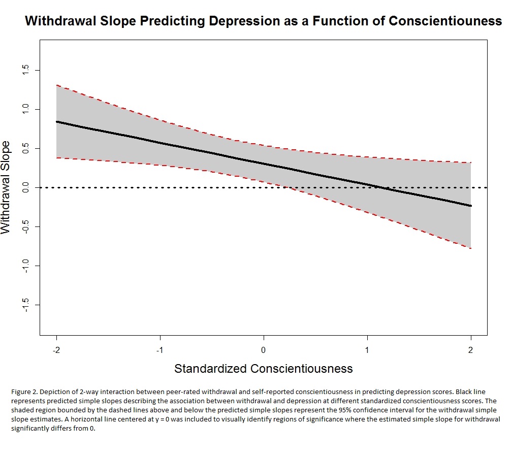
I personally do not like simply presenting the significance of simple slopes at static values, though this is a common practice in my field (behavioral science). Instead, I generally advocate for displaying significance of simple slopes across a comprehensive range of possible moderator values (at least when significant moderation appears to exist).

In the image below, conscientiousness is the moderator and displayed on the x-axis. Simple slopes relating social withdrawal to the outcome are plotted on the y-axis. The shaded region represents the 95% confidence interval for the estimated simple slopes. If zero falls outside the interval for an estimated simple slope (as indicated by the horizontal line), you can conclude that the simple slope at that level of the moderator is statistically significant.