Is it possible to make this GAM even less smooth to generate a better fit?

Question

I have done a logistic regression with two independent variables (x1 and x2) and a dependent binary variable (y). The AUC (roc curve) is 0.7915.

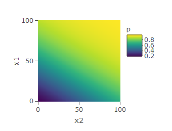
The heatmap below shows the probabilities resulting from the predict function. It seems the logistic regression is not flexible enough since the range of p (probabilities) for x1=10 is 0.25 – 0.76 while in reality this range is 0.25 – 1.

For that reason I have use the GAM - package to create a GAM with smoothing splines.

mygam=gam(y~s(x1,df=100)+s(x2,df=100),family=binomial,data=mydata3)

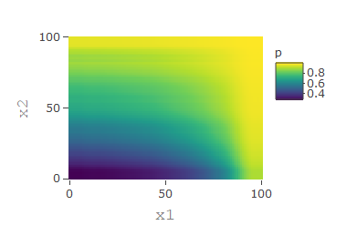
This generates an improvement in AUC to 0.807. The heatmap below shows the probabilities resulting from the GAM-predict function.

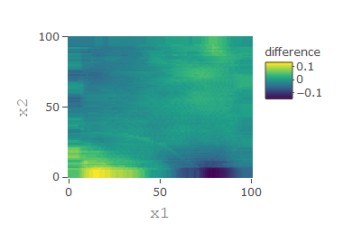
Although there is still an area for x1 between 0 and 10 where the GAM shows large differences in comparison to a Pivot-table of my raw data (for every (x1,x2): count(y==1) / total y). The heatmap below shows the differences between the GAM and the Pivot table:

Even if I set the degrees of freedom higher than 100, this give no improvement. I have also tried lo for local regression although no improvement. I also have tried several settings with mgcv although it seems not possible to make a GAM flexible enough to fit the range for x2 between 0 and 10.

Would there be any possibility to reach the fit with a GAM or is the data to steep?

Thanks a lot!

Ps: only the labels in the first graph are swapped (not the variables).

Answer 1

[I'm going to assume that you are using mgcv as indicated by the mgcv tag; if you aren't, consider switching to it as it provides a much more modern approach to estimating GAMs than the gam package.]

It seems like you want to model a bivariate smooth or smooth interaction between x1 and x2.

If you want to model a smooth interaction between two variables then you can do this via a tensor product smooth in mgcv using either the te() or t2() functions. You can do multivariate smooths with s() but those are isotropic and as such not generally suitable for modelling interactions where the covariates involved in the interaction will typically be measured in different units and on different scales.

With te() or t2() you can set the dimensions of the two marginal bases as required by passing a vector to argument k. By the looks of the output you showed, whilst you are passing it k = 100 for the marginal smooths, the penalised spline estimat is one for a much smoother surface — so you probably don't want to pass k = c(100,100) as that would be a ridiculously complex basis expansion to work with.

mygam <- gam(y ~ te(x1, x2, k = c(20,20)),
             method = 'REML',
             family = binomial, data = mydata3)

This will estimate a smooth interaction (main effects plus interaction) between x1 and x2 with smoothness selection performed using REML, which is preferred over the default GCV. Each marginal basis will use 20 basis functions, for a total of 400 (20*20), although one will be removed due to identifiability constraints with the intercept.

If you want to decompose the smooth interaction into main (marginal) effects and pure interaction then we can use the ti() smoother as follows:

mygam <- gam(y ~ s(x1, k = 20) + s(x2, k = 20) + ti(x1, x2, k = c(10,10)),
             method = 'REML',
             family = binomial, data = mydata3)

where the s() termsdefine the main effects of each variable and the ti() term has has the marginal effects of the full basis (that you'd get withte()`) removed.

The t2() version works like te() but uses a different parameterisation of the tensor product, although an advantage is that it it is easier to decompose the t2() into the two marginal effects and an interaction effect than with te(). The main advantage of t2() is that it can be used with gamm4::gamm4(), whereas te() can't.

All that said, the final graph you show suggests that the data exhibit some thresholds and cut points, which may not be well modelled with a smooth function.

Answer 2

Try something like:

mygam = gam (y ~ s(x1, x2), family=binomial, data=mydata3)

In your original code, I believe you're treating x1 and x2 distinctly rather than jointly. Combining the two into a single smooth may help. You might also want to investigate other smoothers besides s.

Of course, you are using smoothing and things can only be so flexible.