8
$\begingroup$

I am trying to solve this problem on and off for the past couple of months but to no success. This was supposed to be a very small part of my PhD thesis in navigation but I guess I underestimated the problem. It sounded trivial at the beginning, but now I am not so sure.

Lets say we have two ships, each with its own nominal position in 2D coordinates (mean). Due to errors in positioning systems we can only be certain that the ships are within 1 mile of the mean with 95% probability (normal distribution). Given these 2 positions and this probability distribution, what is the probability that the ships are within 5 miles from each other? Also, same question if the ship's probable position is an ellipse, not a circle.

I asked some people and they told me that there are no analytic solutions. If that is really the case, please explain how to solve it numerically.

As you can already tell, I come from engineering background, therefore my math is more than a bit rusty.

I apologize in advance if the question is too vague or too trivial for this forum. I will be more than happy to explain in more detail if needed.

I found this, but it is only for univariate case, and besides I don't know how to implement it in my case where I need to find the probability that the distance between two ships is less than 5 miles.

I imagine this problem as a plane with two hills that intersect and the solution is the volume under the circle with diameter of 5 miles that is located somewhere between the two peaks of hills (means).

Am I on the right track?

Thanks

$\endgroup$
16
  • 3
    $\begingroup$ What positioning systems are the ships using? In some cases (such as GPS), the errors may be correlated, which will affect the calculations. $\endgroup$
    – whuber
    Commented Nov 5, 2012 at 15:39
  • 1
    $\begingroup$ Did I miss the nominal positions of each ship, or do you want a general solution for any pair of positions ? $\endgroup$ Commented Nov 5, 2012 at 18:20
  • 1
    $\begingroup$ I don't think the model of a circular region centered on a point is correct here, as that gives the probability that the two ships are both within a fixed distance of that point. There are many cases when neither ship will be in that region, yet both ships may be close to one another. $\endgroup$ Commented Nov 7, 2012 at 8:20
  • 3
    $\begingroup$ My earlier comment still stands: combining correlated sources of error may produce correlated estimates of position, which will affect the calculations. Although in practice the magnitude of the resulting error may be inconsequential, some analysis of it ought to be offered to justify the solution. Incidentally, this question has no unique answer unless you provide a prior distribution for the ship locations (or at least their mutual distance): that may be why a solution has been eluding you. $\endgroup$
    – whuber
    Commented Nov 12, 2012 at 17:29
  • 2
    $\begingroup$ Sorry about the vagueness: I was thinking of "mutual distance" as a random variable describing the actual positions. My concern is that you might be asking for something you can't get: to derive a probability distribution for the actual ship-to-ship distance based on measurements, you need to update a prior distribution using Bayes' Theorem. If that's not how you're thinking about this problem, you might actually be asking how to compute confidence or prediction intervals. I'm trying to elicit enough information from you to clarify this point, because it may be important. $\endgroup$
    – whuber
    Commented Nov 13, 2012 at 20:45

3 Answers 3

7
$\begingroup$

Summary

The problem is not trivial, but obtaining a solution is straightforward. Exact analytical expressions for the distribution of the inter-ship distance can be found (in terms of Bessel functions): it is the square root of a scaled non-central chi-squared variate. Provided the ships are far apart compared to the standard deviation of the position estimates, formulas for the mean and variance of this distribution provide an excellent Normal approximation. This can be used to develop either confidence intervals or a posterior distribution for the distance.


A comment describes the data:

The data that I have is 2 pairs of x,y coordinates that mark the estimated positions of 2 ships. Also, positional errors are bivariate normal with 95% probability of ship's actual position being within 1 mile of the expected position.

It will be convenient to obtain conventional parameters of the positional errors. A bivariate normal distribution with no correlation and variances of $\sigma^2$ for each of the coordinates has a total probability of $1 - \exp(-x^2/(2\sigma^2))$ within a distance $x$ of its mean. Letting $x$ be one mile and setting this expression to $0.95$ determines $\sigma^2$. In general, when the probability is $1-\alpha$ ($\alpha=0.05$ here) at a radius of $x$, then

$$\sigma^2 = \frac{x^2}{-2 \log(\alpha)}.$$

Let $(X_1,Y_1)$ be the observed location of ship 1, assumed to be at the unknown location $(\mu_{x1}, \mu_{y1})$ and $(X_2,Y_2)$ the observed location of ship 2, assumed to be at $(\mu_{x2}, \mu_{y2})$. Their squared distance,

$$D^2 = (X_1 - X_2)^2 + (Y_1 - Y_2)^2,$$

is a sum of squares of two Normal variates: $X_1-X_2$ has an expectation of $\mu_{x1}-\mu_{x2}$ and a variance of $2\sigma^2 = \sigma^2 + \sigma^2$ while $Y_1-Y_2$ has an expectation of $\mu_{y1}-\mu_{y2}$ and a variance of $2\sigma^2$. This makes $D^2$ equal to $2\sigma^2$ times a non-central $\chi^2$ distribution with $\nu=2$ degrees of freedom and noncentrality parameter

$$\lambda = \frac{(\mu_{x1}-\mu_{x2})^2 + (\mu_{y1}-\mu_{y2})^2}{2\sigma^2}.$$

Consequently, $D$ itself could be called a (scaled) "noncentral $\chi$ distribution."

Calculations indicate that the mean of $D$ equals $\sqrt{2}\sigma$ times $$\frac{1}{2} e^{-\lambda /4} \sqrt{\frac{\pi }{2}} \left((2+\lambda ) \text{BesselI}\left[0,\frac{\lambda }{4}\right]+\lambda \text{BesselI}\left[1,\frac{\lambda }{4}\right]\right)$$ and (somewhat surprisingly) its raw second moment is $2\sigma^2$ times $2+\lambda$. As we would intuitively expect, the mean (upper blue curve) is close to $\sqrt{\lambda}$ (lower red curve), especially for large $\lambda$, which occurs when the ships are well separated:
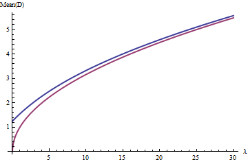
Plot of mean versus lambda

From these, by matching moments, we obtain a Normal approximation to $D$. It is remarkably good when the ships are separated by several $\sigma$'s. (The Normal approximation has slightly shorter tails.) For instance, here are plots of the distribution of $D$ and its Normal approximation when the two ships are actually $5$ miles apart in the circumstances of the initial quotation:
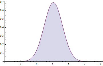
PDF plot and its approximation

At this resolution, they perfectly coincide. The correct probability that $D$ is less than $5$, $\Pr(D\le 5)$, is equal to $0.476912$, while the probability given by the Normal approximation is $0.476807$: just $0.0001$ off.

However, these calculations do not directly answer the question, which is: given the observed value of $D$, what can we say about the true distance between the ships (equal to $\delta = \sqrt{(\mu_{x1}-\mu_{x2})^2 + (\mu_{y1}-\mu_{y2})^2}$)? This usually has two kinds of answers:

  1. For any desired level of confidence, we can compute an associated confidence interval for $\delta$, or

  2. If we adopt a prior distribution for $\delta$, we can update that distribution (via Bayes' Theorem) based on $D$ to obtain a posterior distribution.

Either method is easy and straightforward when the Normal approximation to the distribution of $D$ is good. Both require some heavy computation otherwise--but that is perhaps a discussion for another day.

$\endgroup$
4
  • 1
    $\begingroup$ I intentionally avoided referencing the Wikipedia article on the noncentral chi distribution because it uses a different parameterization! (Its $\lambda$ is the square root of the $\lambda$ used here.) $\endgroup$
    – whuber
    Commented Nov 14, 2012 at 17:29
  • 1
    $\begingroup$ Wow, firstly, I want to thank you for this answer. I am humbled by the effort you invested in writing this, let alone figuring it out. Secondly, as you might have guessed already, I will need some time to digest everything you wrote. Thirdly, now I think I understand where I was wrong while considering this problem. All this time I thought that the observed ships' positions were exactly at the position of their means. Furthermore, I thought that that is how the means are defined in terms of positioning systems. I just figured that the observed position is the center of the error circle. [cont] $\endgroup$
    – mmacx
    Commented Nov 14, 2012 at 21:11
  • $\begingroup$ [cont] After reading your answer for half a dozen times, I am still not sure I completely understand where I was going wrong, but I'll keep trying to figure it out. My mind is doing backflips right now, thank you :) $\endgroup$
    – mmacx
    Commented Nov 14, 2012 at 21:12
  • $\begingroup$ I had to be terse (and wish there were time to provide a more complete answer): feel free to follow up with requests for further clarification. $\endgroup$
    – whuber
    Commented Nov 14, 2012 at 22:01
2
$\begingroup$

I'm not sure how much this will help you but I hope it gives some pointers.

Here is a Mathematica function which computes the probability under the distributions for a circle of radius separation/2 for two ships with a normal distribution of position with variance 0.2. A variance of 0.2 is close to the 95% certainly level.

In brief it defines a mixture distribution in 2 dimensions with covariance matrix {{0.2,0},{0,0.2}} (* other covariance matrices would account for elliptical distributions *). Forms the probability distribution function for that mixture and then numerically integrates it over the required range.

(* Uses absolute separation distance rotated to the x axis *)

probProximity[reportedSeparationMiles_, probabiityRangeMiles_] := 
 With[{dist = MixtureDistribution[{1, 1},
 {MultinormalDistribution[{-(reportedSeparationMiles/2),0}, {{0.2, 0}, {0,0.2}}], 
  MultinormalDistribution[{  reportedSeparationMiles/2, 0}, {{0.2, 0}, {0,0.2}}]}]}, 
  NIntegrate[
   PDF[dist][{x, y}] 
   Boole[Abs[\[Sqrt]((0 - x)^2 + (0 - y)^2)] <= probabiityRangeMiles/2], 
   {x, -(probabiityRangeMiles/2), probabiityRangeMiles/2}, 
   {y, -(probabiityRangeMiles/2), probabiityRangeMiles/2}]]

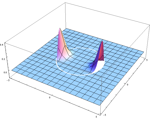
The probability distribution of position for two ships 5 miles apart with a 95% confidence of being within one mile of reported position.

Separation Distribution

For a range of 5 miles, the calculated value is

probProximity[5, 5]

0.464173

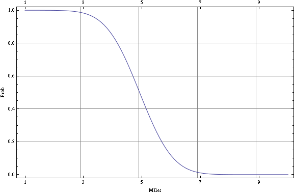
Here is the probability of proximity over a range of distances: Probability of separation

$\endgroup$
6
  • $\begingroup$ Thank you for the excellent reply. I guess this is what I was looking for. It will take me a while until I figure the details of the code since I don't use Mathematica, but in the meantime can you please tell me if the second figure is made with probProximity[n,1] or [n,5]? Also, in your opinion, if these two ships are moving, can I calculate probabilities of loss of separation for each point in time (pairs of coordinates) and use the highest probability as the total measure of probability that they will lose separation? Or should I integrate them somehow? Thanks $\endgroup$
    – mmacx
    Commented Nov 6, 2012 at 11:20
  • 1
    $\begingroup$ @mmacx After reconsidering I'm not yet happy with this answer, it only calculates the probability of the two ships being simultaneously within 5 miles of their midpoint. Because the positions are being modelled with Gaussians, their extent is infinite. So there are many rare configurations where both ships may be far from their nominal positions yet within 5 miles of each other. $\endgroup$ Commented Nov 6, 2012 at 21:50
  • $\begingroup$ Thanks for the follow-up. Shouldn't probabilities of separation loss for each of those pairs of positions be less than the one you calculated above? If so, I'm not interested in those because I wish to find the highest probability. $\endgroup$
    – mmacx
    Commented Nov 6, 2012 at 22:27
  • 1
    $\begingroup$ Just to clarify, the term "separation loss", is when the two ships are closer than five miles? If you are interested in the probability of separation loss over time, just as in the case of throwing a 6 with a die, then the likelihood is not the maximum probability of throwing a 6 in one turn, but a summation of the probability of achieving a 6 in any of n trials. $\endgroup$ Commented Nov 7, 2012 at 8:38
  • 1
    $\begingroup$ @mmacx Nothing seems to be quite that simple with probability :). In the case of the die, the probability is given by the summation according to the Binomial distribution, en.wikipedia.org/wiki/Binomial_distribution. I think an outline solution for your case would be to consider the probability that ship one is at point and then integrate the probability, according to the normal positional distribution that you assume, that ship 2 is within 5 miles of that point. And to repeat that for all points in the 2D space in which the ships can be. $\endgroup$ Commented Nov 7, 2012 at 15:21
1
$\begingroup$

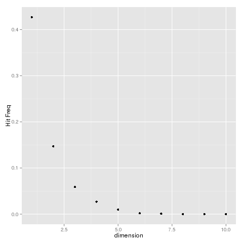
I've thrown up a simulation with R with increasing dimension in response to Erik's answer. This code also answers the question, by providing a numerical solution (when fixing the dimension to 2) to a special case which can be easily generalized (though it's not very efficient).

Erik proposed to look at the problem as a one-dimensional problem by choosing a coordinate system, which lies on the lines connecting the two ships. This can't work, as with increasing dimension, the probability being close decreases.

I'm sampling from two $d$-dimensional Gaussians with means $(1,0,\dots)$ and $(0,0,\dots)$. Covariance is the identity matrix. The code plots the frequency of the points being within 1 of each other (euclidean distance) and uses 1000 samples for each dimension.

Using simulation you can easily model ellipses simply by adjusting the covariance matrix (what my code doesn't allow, since I don't use a library for sampling from gaussians).

require(ggplot2)

euc.dist <- function(x1,x2) {
        d = length(x1)
        sqrt(sum((x1-x2) ^ 2))
}
drawDist <- function(d) {
        v1 <- replicate(d,rnorm(1))
        v2 <- replicate(d,rnorm(1))
        #resample the first component of v1 to get 1,0,0,...
        v1[1] <- rnorm(1,1)
        euc.dist(v1,v2)
}
png("hit-prob.png")
qplot(1:10,
      sapply(1:10,function(d) 
           mean(replicate(1000,drawDist(d) < 1))), #This is the important line
      xlab="dimension",ylab="Hit Freq")
dev.off()

enter image description here

$\endgroup$
2
  • $\begingroup$ Thanks for your answer and code. Can you tell me please, where can I see that comment by @Erik that is now missing. Thanks $\endgroup$
    – mmacx
    Commented Nov 5, 2012 at 20:45
  • $\begingroup$ @mmacx Seems like he deleted it. I'm adding a comment to my answer. $\endgroup$
    – ziggystar
    Commented Nov 12, 2012 at 12:41

Your Answer

By clicking “Post Your Answer”, you agree to our terms of service and acknowledge you have read our privacy policy.

Not the answer you're looking for? Browse other questions tagged or ask your own question.