How can we explain the meaning of some specific coefficients in generalized Difference-in-Difference?

Question

I read a paper using genenalized Difference-in-Difference

$Y_{it}$ = $\alpha$ + $\beta$ $(Leniency Law)_{kt}$ + $\delta$$X_{ikt}$ + $\theta$$_t$ + $\gamma$$_i$ +$\epsilon$$_{it}$

where i,k, and t index firms, countries, and years respectively. $X_{ikt}$ is a vector of the different firm, country, and industry control, while $\gamma$ and $\theta$ are firm and year fixed effects.

The variable of interest here is $(Leniency Law)_{kt}$. Dasgupta,2019,p.2597 documented that this variable equals 0 before the passage of the leniency law in country k, and 1 afterward.

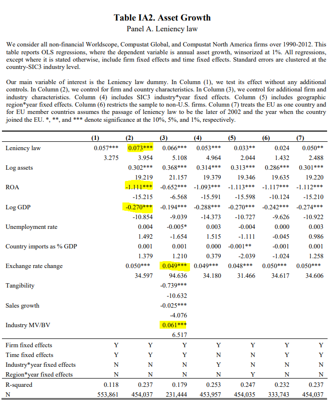
From the Table IA2 in their Appendix, I am wondering how we can interpret the coefficient of some independent variables which are yellowed as below

From my understanding, 0.0073 is explained as: asset growth in treatment countries increase 0.073% compared to the change in asset growth in the control country after anticollusion. I am wondering it is correct and how to explain the rest.

Answer 1

So if I understand this question correctly you are asking about adding controls in the DD. First, let us consider why one would do this. There are essentially two reasons,

1. Reduce Error Variance
2. Aid in Identification

The first reason is simple enough. Adding in covariates helps to explain some of the variation in $Y$ and so reduces the variance in our residuals. This is desirable if we are after significance levels. The second reason is a little more tricky but essentially comes back to the same idea of explaining some of the variation in $Y$. Recall, that we need that the common trends assumptions holds between treatment and control. This is the key identifying assumption. It is possible that when we look at the pre-trends prior to controlling for a covariate we see a failure in common trends. It is possible by adding in the missing covariate we now control for the difference in slope. Notice, covariates only affect identification if they are at the group/time level. There are other more complicated cases to add covariates but I do not think this is relevant here (here is a paper if you are interested).

So now that we know why we do this, let us think about how. Well, we can simply add them to the regression. The main condition is that we really need these to be exogenous (unless of course, we are doing something more complicated like in that linked paper). Given that, if we are after (2) then we want something like,

$$Y_{igt}=\alpha + \beta D_{gt} + \gamma_g + \theta_t + X_{gt}\delta + e_{igt}$$

If we just want to reduce standard errors we can do,

$$Y_{igt}=\alpha + \beta D_{gt} + \gamma_g + \theta_t + X_{igt}\delta + e_{igt}$$

The within-group variation will have no effect on identification but may help lower the standard errors.

In terms of interpretation, we may interpret the $\beta$ as we usually do. The independent covariates do not really matter though unless we are interested in them. They do not affect the interpretation of the treatment effect, though they may allow us to claim better identification. If they are truly exogenous we may interpret them casually, otherwise we interpret them as we normally interpret multiple regression coefficients. So for example, we can interpret the coefficient on ROA as saying that if we held all other variables constant but increased ROA by 1 unit we would expect a -1.111 decline in the outcome, on average. However, in practice, I would caution against assigning too much weight to these coefficients because often the authors include them to reduce standard errors and are not the variables of interest. Finally, here are a set of notes by Pischke on DID that include adding covariates. And, here is another set by Wooldridge. Perhaps, these will be helpful for you.