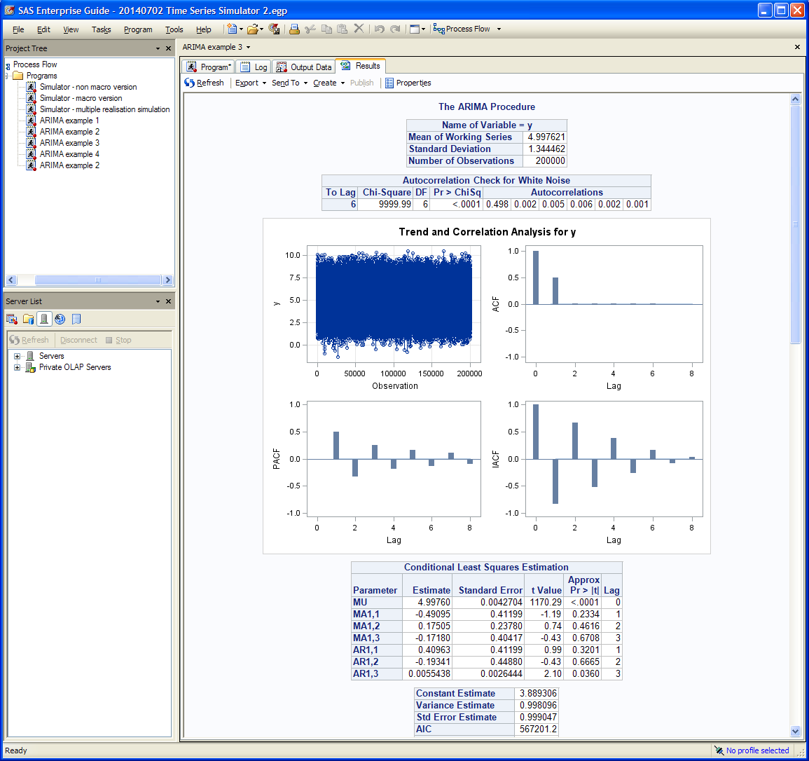
Interesting exercise. I think that rather than using a few long series (200,000 observations), it would be more informative to use several shorter series (e.g. 5,000 series of 200 observations) and see what we find on average. I carried out a small exercise that can be reproduced with the R code posted at the end of this answer.
A MA can be approximated by an AR process, after all, an AR model consists of weights of past observations, which include the innovations that configure the MA term. Thus, significant AR coefficients may be expected. Significant MA(2) and MA(3) observed at a high rate would be more strange to me.
In this small exercise, when the ARMA(0,0,1) was used to generate the data, the AR and MA coefficients of the ARMA(3,0,3) model were found to be significant in 60%-70% of cases (the null of zero coefficient is rejected for a critical value set to 2). The AR(3) coefficient behaved differently, it was significant only in around 11% of cases. The MA coefficients were found significant in a few more cases than the AR coefficients. No major differences in significance rates were observed across the MA coefficients. This is not exactly in line with the expected results that I mentioned above, but agrees with your findings than AR and MA coefficients that are not part of the data generating process can turn out to be significant in several cases.
I also compared the AIC and BIC from each fitted model. The AIC chose the right model (the ARMA(0,0,1) used to generate the data) in 53% of cases and the BIC around 74% of cases. Using a MA coefficient equal to 0.6 (and hence farther from the non-invertible MA with unit coefficient) I observed similar results.
This small exercise suggests using the BIC when it comes to choosing an ARMA model. As suggested also by your exercise, tests for significance of the coefficients can sometimes be deceptive.
You may be interested in these posts here and here. My answers to those posts discuss a related issue.
R code:
Parameters of the exercise:
niter <- 5000       # number of iterations
n <- 200            # number of observations in each series
ma.coef <- 0.9      # MA coefficient for the data generating process ARIMA(0,0,1)
                    # (try other values not so close to a non-invertible MA)
morder2 <- c(3,0,3) # order of the model to be compared with the ARMA(0,0,1)
cval <- 2           # critical value to determine the significance of ARMA coefficients
Main code:
set.seed(123)
rejections <- rep(0, sum(morder2[-2]))
aic.choices <- bic.choices <- rep(NA, niter)
na <- 0
k2 <- sum(morder2[-2]) + 1
for (i in seq.int(niter))
{
  x <- arima.sim(n = n, model = list(order = c(0,0,1), ma = ma.coef))
  fit1 <- try(arima(x, order = morder2, include.mean = FALSE), silent = TRUE)
  if (!inherits(fit1, "try-error"))
  {
    sde <- sqrt(diag(fit1$var.coef))
    if (anyNA(sde)) {
      na <- na + 1
    } else {
      tstats <- abs(coef(fit1)) / sde
      rejections <- rejections + as.numeric(tstats > cval)
    }
    aic.choices[i] <- which.min(c(AIC(fit1), AIC(fit2)))
    bic.choices[i] <- which.min(c(AIC(fit1) - 2*k2 + k2 * log(n),
      AIC(fit2) - 4 + 2 * log(n)))
  } else
    na <- na + 1
  fit2 <- arima(x, order = c(0,0,1), include.mean = FALSE)
}
names(rejections) <- names(coef(fit1))
Results for ma.coef=0.9:
rejections / (niter - na)
#       ar1       ar2       ar3       ma1       ma2       ma3
# 0.6076359 0.7107420 0.1059103 0.6814064 0.7118205 0.7180759
na
# [1] 364
table(aic.choices, useNA = "always") / niter
#      1      2   <NA>
# 0.4560 0.5338 0.0102
table(bic.choices, useNA = "always") / niter
#      1      2   <NA>
# 0.2504 0.7394 0.0102

