220
$\begingroup$

Here is the article that motivated this question: Does impatience make us fat?

I liked this article, and it nicely demonstrates the concept of “controlling for other variables” (IQ, career, income, age, etc) in order to best isolate the true relationship between just the 2 variables in question.

Can you explain to me how you actually control for variables on a typical data set?

E.g., if you have 2 people with the same impatience level and BMI, but different incomes, how do you treat these data? Do you categorize them into different subgroups that do have similar income, patience, and BMI? But, eventually there are dozens of variables to control for (IQ, career, income, age, etc) How do you then aggregate these (potentially) 100’s of subgroups? In fact, I have a feeling this approach is barking up the wrong tree, now that I’ve verbalized it.

Thanks for shedding any light on something I've meant to get to the bottom of for a few years now...!

$\endgroup$
17
  • 5
    $\begingroup$ Epi & Bernd, Thanks so much for trying to answer this. Unfortunately, these answers are a big leap from my question, and are over my head. Maybe it' b/c I don't have experience with R, and just a basic Statistics 101 foundation. Just as feedback to your teaching, once you abstracted away from BMI, age, impatience, etc to "covariate" et al, you totally lost me. Auto-generating pseudo-data also was not helpful in clarifying the concepts. In fact, it made it worse. It's hard to learn on dummy data with no inherent meaning, unless you already know the principle being explained (ie: Teacher knows i $\endgroup$
    – JackOfAll
    Commented Oct 23, 2011 at 23:20
  • 9
    $\begingroup$ Thanks for asking this question of fundamental importance, @JackOfAll - the site would be incomplete without a question along these lines - I've 'favorited' this one. The answers here have been very helpful to me and apparently many others based on the number of upvotes. If, after pondering this, you've found the answers helpful yourself (or the answers to any of your questions), I encourage you to use your upvotes and to accept an answer if you find it definitive. This can be done by clicking the little upward pointing bell curves next the answer and the checkmark, respectively. $\endgroup$
    – Macro
    Commented Jul 24, 2012 at 22:53
  • 4
    $\begingroup$ This is not a complete answer or anything, but I think it's worthwhile to read "Let's Put Garbage-Can Regressions and Garbage-Can Probits Where They Belong" by Chris Achen. (PDF link: http://qssi.psu.edu/files/Achen_GarbageCan.pdf) This applies to both Bayesian and Frequentist approaches equally. Just throwing terms into your set-up is not sufficient to "control" for effects, but sadly this is what passes for control in a lot of the literature. $\endgroup$
    – ely
    Commented Oct 5, 2012 at 19:41
  • 9
    $\begingroup$ You ask "how the computer software controls for all variables at the same time mathematically". You also say "I need an answer that does not involve formulas". I don't see how it's possible to really do both at the same time. At least not without serious risk of leaving you with flawed intuition. $\endgroup$
    – Glen_b
    Commented Jul 13, 2014 at 10:21
  • 3
    $\begingroup$ I'm surprised this question has not gotten more attention. I agree with the OP's comment that other questions on the site do not exactly cover the specific issue that is brought up here. @Jen, the very short answer to your (second) question is that the multiple covariates really are partialed out simultaneously and not iteratively as you describe. Now I will think about what a more detailed and intuitive answer to these questions would look like. $\endgroup$ Commented Aug 25, 2014 at 19:03

5 Answers 5

180
$\begingroup$

There are many ways to control for variables.

The easiest, and one you came up with, is to stratify your data so you have sub-groups with similar characteristics - there are then methods to pool those results together to get a single "answer". This works if you have a very small number of variables you want to control for, but as you've rightly discovered, this rapidly falls apart as you split your data into smaller and smaller chunks.

A more common approach is to include the variables you want to control for in a regression model. For example, if you have a regression model that can be conceptually described as:

BMI = Impatience + Race + Gender + Socioeconomic Status + IQ

The estimate you will get for Impatience will be the effect of Impatience within levels of the other covariates - regression allows you to essentially smooth over places where you don't have much data (the problem with the stratification approach), though this should be done with caution.

There are yet more sophisticated ways of controlling for other variables, but odds are when someone says "controlled for other variables", they mean they were included in a regression model.

Alright, you've asked for an example you can work on, to see how this goes. I'll walk you through it step by step. All you need is a copy of R installed.

First, we need some data. Cut and paste the following chunks of code into R. Keep in mind this is a contrived example I made up on the spot, but it shows the process.

covariate <- sample(0:1, 100, replace=TRUE)
exposure  <- runif(100,0,1)+(0.3*covariate)
outcome   <- 2.0+(0.5*exposure)+(0.25*covariate)

That's your data. Note that we already know the relationship between the outcome, the exposure, and the covariate - that's the point of many simulation studies (of which this is an extremely basic example. You start with a structure you know, and you make sure your method can get you the right answer.

Now then, onto the regression model. Type the following:

lm(outcome~exposure)

Did you get an Intercept = 2.0 and an exposure = 0.6766? Or something close to it, given there will be some random variation in the data? Good - this answer is wrong. We know it's wrong. Why is it wrong? We have failed to control for a variable that effects the outcome and the exposure. It's a binary variable, make it anything you please - gender, smoker/non-smoker, etc.

Now run this model:

lm(outcome~exposure+covariate)

This time you should get coefficients of Intercept = 2.00, exposure = 0.50 and a covariate of 0.25. This, as we know, is the right answer. You've controlled for other variables.

Now, what happens when we don't know if we've taken care of all of the variables that we need to (we never really do)? This is called residual confounding, and its a concern in most observational studies - that we have controlled imperfectly, and our answer, while close to right, isn't exact. Does that help more?

$\endgroup$
11
  • 1
    $\begingroup$ Thanks. Anyone know a simple example regression based example online or in a textbook that I can work through? $\endgroup$
    – JackOfAll
    Commented Oct 20, 2011 at 21:47
  • 1
    $\begingroup$ @JackOfAll There are likely hundreds of such examples - what areas/types of questions are you interested in, and what software packages can you use? $\endgroup$
    – Fomite
    Commented Oct 20, 2011 at 21:49
  • 14
    $\begingroup$ +1 For answering this without the negativity that I would use. :) In typical parlance, controlling for other variables means the authors threw them into the regression. It doesn't really mean what they think it means if they have not validated that the variables are relatively independent and that the entire model structure (usually some kind of GLM) is well-founded. In short, my view is that whenever someone uses this phrase, it means they have very little clue about statistics, and one should re-calculate the results using the stratification method you offered. $\endgroup$
    – Iterator
    Commented Oct 22, 2011 at 12:49
  • 7
    $\begingroup$ @SibbsGambling You will note that the original questioner asked for a simple worked example. $\endgroup$
    – Fomite
    Commented Mar 31, 2015 at 5:04
  • 1
    $\begingroup$ @Fomite: you state "There are many ways to control for variables. The easiest, and one you came up with, is to stratify your data so you have sub-groups with similar characteristics - there are then methods to pool those results together to get a single "answer"." I've posted a question stats.stackexchange.com/questions/380755/… asking people to explain stratification and aggregation and the sense I am getting from the lack of response and a couple comments is that it is not possible. Please show us the way. $\endgroup$ Commented Dec 10, 2018 at 22:10
68
$\begingroup$
  1. Introduction

    I like @EpiGrad's answer (+1) but let me take a different perspective. In the following I am referring to this PDF document: "Multiple Regression Analysis: Estimation", which has a section on "A 'Partialling Out' Interpretation of Multiple Regression" (p. 83f.). Unfortunately, I have no idea who is the author of this chapter and I will refer to it as REGCHAPTER. A similar explanation can be found in Kohler/Kreuter (2009) "Data Analysis Using Stata", chapter 8.2.3 "What does 'under control' mean?".

    I will use @EpiGrad's example to explain this approach. R code and results can be found in the Appendix.

    It also should be noted that "controling for other variables" does only make sense when the explanatory variables are moderately correlated (collinearity). In the aforementioned example, the Product-Moment correlation between exposure and covariate is 0.50, i.e.,

    > cor(covariate, exposure)
    [1] 0.5036915
    
  2. Residuals

    I assume that you have a basic understanding of the concept of residuals in regression analysis. Here is the Wikipedia explanation: " If one runs a regression on some data, then the deviations of the dependent variable observations from the fitted function are the residuals".

  3. What does 'under control' mean?

    Controlling for the variable covariate, the effect (regression weight) of exposure on outcome can be described as follows (I am sloppy and skip most indices and all hats, please refer to the above mentioned text for a precise description):

    $\newcommand{\resid}{{\rm resid}}\newcommand{\covariate}{{\rm covariate}}$ $$\beta_1=\frac{\sum \resid_{i1} \cdot y_i}{\sum \resid^2_{i1}}$$

    $\resid_{i1}$ are the residuals when we regress exposure on covariate, i.e.,

    $${\rm exposure} = {\rm const.} + \beta_{\covariate} \cdot \covariate + \resid$$

    The "residuals [..] are the part of $x_{i1}$ that is uncorrelated with $x_{i2}$. [...] Thus, $\hat{\beta}_1$ measures the sample relationship between $y$ and $x_1$ after $x_2$ has been partialled out" (REGCHAPTER 84). "Partialled out" means "controlled for".

    I will demonstrate this idea using @EpiGrad's example data. First, I will regress exposure on covariate. Since I am only interested in the residuals lmEC.resid, I omit the output.

    summary(lmEC <- lm(exposure ~ covariate))
    lmEC.resid   <- residuals(lmEC)
    

    The next step is to regress outcome on these residuals (lmEC.resid):

    [output omitted]
    
    Coefficients:
                Estimate Std. Error t value Pr(>|t|)    
    (Intercept)  2.45074    0.02058 119.095  < 2e-16 ***
    lmEC.resid   0.50000    0.07612   6.569 2.45e-09 ***
    ---
    Signif. codes:  0 ‘***’ 0.001 ‘**’ 0.01 ‘*’ 0.05 ‘.’ 0.1 ‘ ’ 1 
    
    [output omitted]
    

    As you can see, the regression weight for lmEC.resid (see column Estimate, $\beta_{lmEC.resid}=0.50$) in this simple regression is equal to the multiple regression weight for covariate, which also is $0.50$ (see @EpiGrad's answer or the R output below).

Appendix

R Code

set.seed(1)
covariate <- sample(0:1, 100, replace=TRUE)
exposure <- runif(100,0,1)+(0.3*covariate)
outcome <- 2.0+(0.5*exposure)+(0.25*covariate)

## Simple regression analysis
summary(lm(outcome ~ exposure))

## Multiple regression analysis
summary(lm(outcome ~ exposure + covariate))

## Correlation between covariate and exposure
cor(covariate, exposure)

## "Partialling-out" approach
## Regress exposure on covariate
summary(lmEC <- lm(exposure ~ covariate))
## Save residuals
lmEC.resid <- residuals(lmEC)
## Regress outcome on residuals
summary(lm(outcome ~ lmEC.resid))

## Check formula
sum(lmEC.resid*outcome)/(sum(lmEC.resid^2))

R Output

> set.seed(1)
> covariate <- sample(0:1, 100, replace=TRUE)
> exposure <- runif(100,0,1)+(0.3*covariate)
> outcome <- 2.0+(0.5*exposure)+(0.25*covariate)
> 
> ## Simple regression analysis
> summary(lm(outcome ~ exposure))

Call:
lm(formula = outcome ~ exposure)

Residuals:
      Min        1Q    Median        3Q       Max 
-0.183265 -0.090531  0.001628  0.085434  0.187535 

Coefficients:
            Estimate Std. Error t value Pr(>|t|)    
(Intercept)  1.98702    0.02549   77.96   <2e-16 ***
exposure     0.70103    0.03483   20.13   <2e-16 ***
---
Signif. codes:  0 ‘***’ 0.001 ‘**’ 0.01 ‘*’ 0.05 ‘.’ 0.1 ‘ ’ 1 

Residual standard error: 0.109 on 98 degrees of freedom
Multiple R-squared: 0.8052,     Adjusted R-squared: 0.8032 
F-statistic: 405.1 on 1 and 98 DF,  p-value: < 2.2e-16 

> 
> ## Multiple regression analysis
> summary(lm(outcome ~ exposure + covariate))

Call:
lm(formula = outcome ~ exposure + covariate)

Residuals:
       Min         1Q     Median         3Q        Max 
-7.765e-16 -7.450e-18  4.630e-18  1.553e-17  4.895e-16 

Coefficients:
             Estimate Std. Error   t value Pr(>|t|)    
(Intercept) 2.000e+00  2.221e-17 9.006e+16   <2e-16 ***
exposure    5.000e-01  3.508e-17 1.425e+16   <2e-16 ***
covariate   2.500e-01  2.198e-17 1.138e+16   <2e-16 ***
---
Signif. codes:  0 ‘***’ 0.001 ‘**’ 0.01 ‘*’ 0.05 ‘.’ 0.1 ‘ ’ 1 

Residual standard error: 9.485e-17 on 97 degrees of freedom
Multiple R-squared:     1,      Adjusted R-squared:     1 
F-statistic: 3.322e+32 on 2 and 97 DF,  p-value: < 2.2e-16 

> 
> ## Correlation between covariate and exposure
> cor(covariate, exposure)
[1] 0.5036915
> 
> ## "Partialling-out" approach
> ## Regress exposure on covariate
> summary(lmEC <- lm(exposure ~ covariate))

Call:
lm(formula = exposure ~ covariate)

Residuals:
     Min       1Q   Median       3Q      Max 
-0.49695 -0.24113  0.00857  0.21629  0.46715 

Coefficients:
            Estimate Std. Error t value Pr(>|t|)    
(Intercept)  0.51003    0.03787  13.468  < 2e-16 ***
covariate    0.31550    0.05466   5.772  9.2e-08 ***
---
Signif. codes:  0 ‘***’ 0.001 ‘**’ 0.01 ‘*’ 0.05 ‘.’ 0.1 ‘ ’ 1 

Residual standard error: 0.2731 on 98 degrees of freedom
Multiple R-squared: 0.2537,     Adjusted R-squared: 0.2461 
F-statistic: 33.32 on 1 and 98 DF,  p-value: 9.198e-08 

> ## Save residuals
> lmEC.resid <- residuals(lmEC)
> ## Regress outcome on residuals
> summary(lm(outcome ~ lmEC.resid))

Call:
lm(formula = outcome ~ lmEC.resid)

Residuals:
    Min      1Q  Median      3Q     Max 
-0.1957 -0.1957 -0.1957  0.2120  0.2120 

Coefficients:
            Estimate Std. Error t value Pr(>|t|)    
(Intercept)  2.45074    0.02058 119.095  < 2e-16 ***
lmEC.resid   0.50000    0.07612   6.569 2.45e-09 ***
---
Signif. codes:  0 ‘***’ 0.001 ‘**’ 0.01 ‘*’ 0.05 ‘.’ 0.1 ‘ ’ 1 

Residual standard error: 0.2058 on 98 degrees of freedom
Multiple R-squared: 0.3057,     Adjusted R-squared: 0.2986 
F-statistic: 43.15 on 1 and 98 DF,  p-value: 2.45e-09 

> 
> ## Check formula
> sum(lmEC.resid*outcome)/(sum(lmEC.resid^2))
[1] 0.5
> 
$\endgroup$
3
  • 7
    $\begingroup$ That chapter looks like Baby Wooldridge (aka Introductory Econometrics: A Modern Approach by Jeffrey M. Wooldridge) $\endgroup$
    – dimitriy
    Commented Oct 6, 2012 at 0:29
  • 5
    $\begingroup$ I may be misunderstanding something, but why don't you need to regress the outcome on covariate as well and then finally regress the outcome residuals on the exposure residuals? $\endgroup$
    – Hank Lin
    Commented Feb 13, 2019 at 17:17
  • 1
    $\begingroup$ @hlinee is right. Can you explain why you don't do this? $\endgroup$ Commented Jul 30, 2019 at 0:34
57
$\begingroup$

Of course some math will be involved, but it's not much: Euclid would have understood it well. All you really need to know is how to add and rescale vectors. Although this goes by the name of "linear algebra" nowadays, you only need to visualize it in two dimensions. This enables us to avoid the matrix machinery of linear algebra and focus on the concepts.


A Geometric Story

In the first figure, $y$ is the sum of $y_{\cdot 1}$ and $\alpha x_1$. (A vector $x_1$ scaled by a numeric factor $\alpha$; Greek letters $\alpha$ (alpha), $\beta$ (beta), and $\gamma$ (gamma) will refer to such numerical scale factors.)
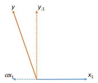
Figure 1

This figure actually began with the original vectors (shown as solid lines) $x_1$ and $y$. The least-squares "match" of $y$ to $x_1$ is found by taking the multiple of $x_1$ that comes closest to $y$ in the plane of the figure. That's how $\alpha$ was found. Taking this match away from $y$ left $y_{\cdot 1}$, the residual of $y$ with respect to $x_1$. ( The dot "$\cdot$" will consistently indicate which vectors have been "matched," "taken out," or "controlled for.")

We can match other vectors to $x_1$. Here is a picture where $x_2$ was matched to $x_1$, expressing it as a multiple $\beta$ of $x_1$ plus its residual $x_{2\cdot 1}$:
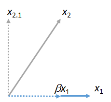
Figure 2

(It does not matter that the plane containing $x_1$ and $x_2$ could differ from the plane containing $x_1$ and $y$: these two figures are obtained independently of each other. All they are guaranteed to have in common is the vector $x_1$.) Similarly, any number of vectors $x_3, x_4, \ldots$ can be matched to $x_1$.

Now consider the plane containing the two residuals $y_{\cdot 1}$ and $x_{2 \cdot 1}$. I will orient the picture to make $x_{2\cdot 1}$ horizontal, just as I oriented the previous pictures to make $x_1$ horizontal, because this time $x_{2\cdot 1}$ will play the role of matcher:
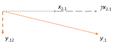
Figure 3

Observe that in each of the three cases, the residual is perpendicular to the match. (If it were not, we could adjust the match to get it even closer to $y$, $x_2$, or $y_{\cdot 1}$.)

The key idea is that by the time we get to the last figure, both vectors involved ($x_{2\cdot 1}$ and $y_{\cdot 1}$) are already perpendicular to $x_1$, by construction. Thus any subsequent adjustment to $y_{\cdot 1}$ involves changes that are all perpendicular to $x_1$. As a result, the new match $\gamma x_{2\cdot 1}$ and the new residual $y_{\cdot 12}$ remain perpendicular to $x_1$.

(If other vectors are involved, we would proceed in the same way to match their residuals $x_{3\cdot 1}, x_{4\cdot 1}, \ldots$ to $x_2$.)

There is one more important point to make. This construction has produced a residual $y_{\cdot 12}$ which is perpendicular to both $x_1$ and $x_2$. This means that $y_{\cdot 12}$ is also the residual in the space (three-dimensional Euclidean realm) spanned by $x_1, x_2,$ and $y$. That is, this two-step process of matching and taking residuals must have found the location in the $x_1, x_2$ plane that is closest to $y$. Since in this geometric description it does not matter which of $x_1$ and $x_2$ came first, we conclude that if the process had been done in the other order, starting with $x_2$ as the matcher and then using $x_1$, the result would have been the same.

(If there are additional vectors, we would continue this "take out a matcher" process until each of those vectors had had its turn to be the matcher. In every case the operations would be the same as shown here and would always occur in a plane.)


Application to Multiple Regression

This geometric process has a direct multiple regression interpretation, because columns of numbers act exactly like geometric vectors. They have all the properties we require of vectors (axiomatically) and therefore can be thought of and manipulated in the same way with perfect mathematical accuracy and rigor. In a multiple regression setting with variables $X_1$, $X_2, \ldots$, and $Y$, the objective is to find a combination of $X_1$ and $X_2$ (etc) that comes closest to $Y$. Geometrically, all such combinations of $X_1$ and $X_2$ (etc) correspond to points in the $X_1, X_2, \ldots$ space. Fitting multiple regression coefficients is nothing more than projecting ("matching") vectors. The geometric argument has shown that

  1. Matching can be done sequentially and

  2. The order in which matching is done does not matter.

The process of "taking out" a matcher by replacing all other vectors by their residuals is often referred to as "controlling" for the matcher. As we saw in the figures, once a matcher has been controlled for, all subsequent calculations make adjustments that are perpendicular to that matcher. If you like, you may think of "controlling" as "accounting (in the least square sense) for the contribution/influence/effect/association of a matcher on all the other variables."


References

You can see all this in action with data and working code in the answer at https://stats.stackexchange.com/a/46508. That answer might appeal more to people who prefer arithmetic over plane pictures. (The arithmetic to adjust the coefficients as matchers are sequentially brought in is straightforward nonetheless.) The language of matching is from Fred Mosteller and John Tukey.

$\endgroup$
3
  • 3
    $\begingroup$ More illustrations along these lines can be found in Wicken's book "The Geometry of Multivariate Statistics" (1994). Some examples are in this answer. $\endgroup$
    – caracal
    Commented Aug 26, 2014 at 7:39
  • 3
    $\begingroup$ @Caracal Thank you for the references. I originally envisioned an answer that uses diagrams like those in your answer--which make a wonderful supplement to my answer here--but after creating them felt that pseudo-3D figures might be too complex and ambiguous to be entirely suitable. I was pleased to find that the argument could be reduced entirely to the simplest vector operations in the plane. It may also be worth pointing out that a preliminary centering of the data is unnecessary, because that is handled by including a nonzero constant vector among the $x_i$. $\endgroup$
    – whuber
    Commented Aug 26, 2014 at 13:12
  • 1
    $\begingroup$ I love this answer because it gives much more intuition than algebra. BTW, not sure if you checked this guy's youtube channel. I enjoyed it a lot $\endgroup$
    – Haitao Du
    Commented Jan 23, 2018 at 17:16
8
$\begingroup$

There is an excellent discussion so far of covariate adjustment as a means of "controlling for other variables". But I think that is only part of the story. In fact, there are many (other) design, model, and machine learning based strategies to address the impact of a number of possible confounding variables. This is a brief survey of some of the most important (non-adjustment) topics. While adjustment is the most widely used means of "controlling" for other variables, I think a good statistician should have an understanding of what it does (and doesn't do) in the context of other processes and procedures.

Matching:

Matching is a method of designing a paired analysis where observations are grouped into sets of 2 who are otherwise similar in their most important aspects. For instance, you might sample two individuals who are concordant in their education, income, professional tenure, age, marital status, (etc. etc.) but who are discordant in terms of their impatience. For binary exposures, the simple paired-t test suffices to test for a mean difference in their BMI controlling for all the matching features. If you are modeling a continuous exposure, an analogous measure would be a regression model through the origin for the differences. See Carlin 2005

$$E[Y_1 - Y_2] = \beta_0 (X_1 - X_2)$$

Weighting

Weighting is yet another univariate analysis which models the association between a continuous or binary predictor $X$ and an outcome $Y$ so that the distribution of exposure levels is homogeneous between groups. These results are typically reported as standardized such as age-standardized mortality for two countries or several hospitals. Indirect standardization calculates an expected outcome distribution from the rates obtained in a "control" or "healthy" population that is projected to the distribution of strata in the referent population. Direct standardization goes the other way. These methods are typically used for a binary outcome. Propensity score weighting accounts of the probability of a binary exposure and controls for those variables in that regard. It is similar to direct standardization for an exposure. See Rothman, Modern Epidemiology 3rd edition.

Randomization and Quasirandomization

It's a subtle point, but if you are actually able to randomize people to a certain experimental condition, then the impact of other variables is mitigated. It's a remarkably stronger condition, because you do not even need to know what those other variables are. In that sense, you have "controlled" for their influence. This is not possible in observational research, but it turns out that propensity score methods create a simple probabilistic measure for exposure that allows one to weight, adjust, or match participants so that they can be analyzed in the same fashion as a quasi-randomized study. See Rosenbaum, Rubin 1983.

Microsimulation

Another way of simulating data that might have been obtained from a randomized study is to perform microsimulation. Here, one can actually turn their attention to larger and more sophisticated, machine learning like models. A term which Judea Pearl has coined that I like is "Oracle Models": complex networks which are capable of generating predictions and forecast for a number of features and outcomes. It turns out one can "fold down" the information of such an oracle model to simulate outcomes in a balanced cohort of people who represent a randomized cohort, balanced in their "control variable" distribution, and using simple t-test routines to assess the magnitude and precision of possible differences. See Rutter , Zaslavsky, and Feuer 2012

Matching, weighting, and covariate adjustment in a regression model all estimate the same associations, and thus all can be claimed to be ways of "controlling" for other variables.

$\endgroup$
5
  • $\begingroup$ Totally over my head. $\endgroup$
    – JackOfAll
    Commented Apr 8, 2018 at 13:27
  • 1
    $\begingroup$ It's an answer to the question that was asked, the good discussion so far is somewhat one-sided in favor of adjustment in multivariate models. $\endgroup$
    – AdamO
    Commented May 16, 2018 at 20:20
  • $\begingroup$ Multivariate models, matching, etc. are all valid techniques, but when does a researcher typically use one technique over another? $\endgroup$
    – mnmn
    Commented Aug 14, 2019 at 13:05
  • $\begingroup$ IS there any good course/MOOC/book on these topics? $\endgroup$
    – aghd
    Commented Jan 29, 2020 at 5:46
  • $\begingroup$ @mnmn matching is most easily achieved by-design: i.e. participant's recruited based on correlatedness (such as twins) or risk-stratification (such as lung cancer patients to non-lung cancer patients based on smoking status). You can also use it to reduce the size of large datasets, so that the statistics are more appealing to the audience. $\endgroup$
    – AdamO
    Commented Sep 23, 2022 at 17:41
0
$\begingroup$

The software doesn't literally control for variables. If you're familiar with matrix notation of regression $Y=X\beta+\varepsilon$, then you may remember that least squares solution is $b=(X^TX)^{-1}X^TY$. So, the software evaluates this expression numerically using computational linear algebra methods.

$\endgroup$
2
  • 4
    $\begingroup$ Thanks for taking the opportunity to offer this information. For the answer to address the needs that are given in the question, we would need to know the meaning of the prime in the second expression and the meaning of the second expression. I understand that slope is the change in one axis over the change in the other. Remember, notation is a special language that was originally created and learned using non notational vocabulary. Reaching people who don't know that language requires using other words and that is the ongoing challenge of bringing knowledge across disciplines. $\endgroup$
    – Jen
    Commented Jul 13, 2014 at 14:29
  • 2
    $\begingroup$ Once you go into multivariate regressions, there's no way to proceed without linear algebra. The Wiki link has all the descriptions of the variables. Here, I can say that $X'$ denots a transpose of $X$ matrix. You'd have to learn how the design matrix is constructed. It's too long to explain it here. Read Wiki which I posted, it has a lot of information. Unless, you understand linear algebra, you will not be able to answer your question in a meaningful way, I'm afraid. $\endgroup$
    – Aksakal
    Commented Jul 13, 2014 at 14:34

Not the answer you're looking for? Browse other questions tagged or ask your own question.