This doesn't read like you are asking for someone to complete a homework question for you, so I will be more generous than @Dilip and give you something of a solution. Wikipedia's article on the likelihood function starts like this:
The likelihood of a set of parameter values, $\theta$, given outcomes
$x$, is equal to the probability of those observed outcomes given
those parameter values
So your confusion is entirely understandable, because that summary is incorrect for continuous distributions. Later on the page it points out that you should use the probability density function instead of the probability function, if your variable is continuous.
In fact, each observed value is modelled as an independent, indentically distributed observation from the uniform distribution, $X \sim U(-a, a)$, which has PDF $\frac{1}{2a}$ for $x \in [-a,a]$ and zero otherwise. Your sample can be regarded as a single observation from a multivariate uniform distribution - effectively a vector, each of whose components (independently) have that uniform distribution. The joint probability density function for that vector of observations is, by independence, the product of the probability density functions for the individual sample observations. To perform maximum likelihood estimation, it is this joint density that we wish to maximise.
For your sample, $x_1 = 12$ and $x_2 = 30$, which I am regarding as a vector of observations, $\vec{x} = \begin{pmatrix} 12 \\ 30 \end{pmatrix}$. The likelihood function is the joint density, i.e. $\mathcal{L}(a|\vec{x}) = f_a(\vec{x})$. Rather than jump straight to how to find the answer, I want to explore a couple of values of $a$ that I hope you will find insightful.
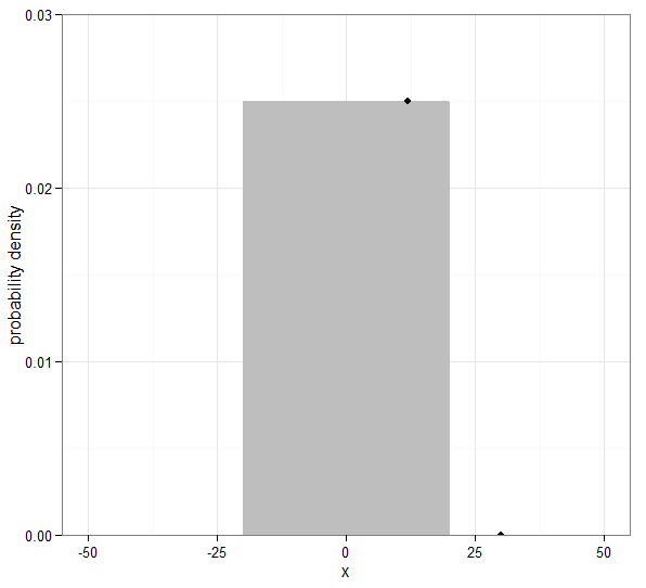
Try $a=20$
The PDF of the uniform distribution will be $\frac{1}{40}=0.025$ for $x \in [-20, 20]$ and $0$ otherwise. The probability density of $x_1 = 12$ will be $0.025$ and of $x_2$ will be $0$, so the joint density of the sample will be $0.025 \times 0 = 0$. We have made the uniform distribution too narrow, so that one of our observed values is impossible, and the likelihood of this choice of parameter is therefore 0. We need to try a bigger value of $a$.

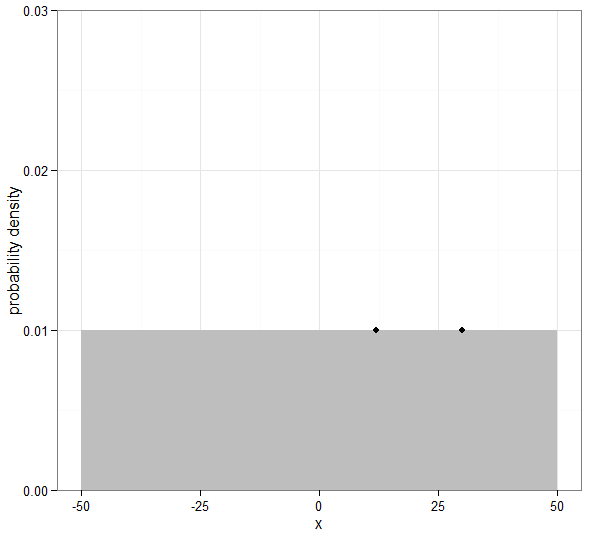
Try $a=50$
The PDF of the uniform distribution will be $\frac{1}{100} = 0.01$ for $x \in [-50, 50]$ and $0$ otherwise. The probability density of $x_1 = 12$ will be $0.01$, and so will be the probability density of $x_2=30$. The joint density will be $0.01 \times 0.01 = 0.0001$ or $\frac{1}{10000}$.

Can we do any better than this? At least this time the likelihood was more than zero. But it is small because our probability densities were small, and this happened because the uniform distribution's probability was spread out over a wider interval (the set of values for which the PDF is above zero, known as the "support"). Let's try narrowing that interval.
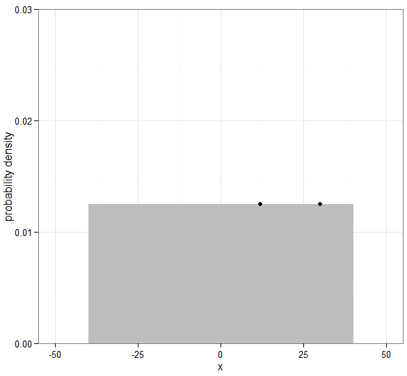
Try $a=40$
The PDF of the uniform distribution will be $\frac{1}{80} = 0.0125$ for $x \in [-40, 40]$ and $0$ otherwise. The probability density of $x_1 = 12$ will be $0.0125$, and so will be the probability density of $x_2=30$. The joint density will be $0.0125 \times 0.0125 = 0.00015625$ or $\frac{1}{6400}$. This is an improvement!

Can we do any better? We would like to make the joint density as high as possible in order to maximise the likelihood, and that means making the PDF of the uniform distribution higher. To achieve that, we want to use a narrower interval. But we already saw that if we made the interval too narrow, the likelihood becomes zero because it makes one of our observations impossible. How narrow can we make $[-a, a]$ before either $x_1=12$ or $x_2=30$ become impossible? Since our distribution is symmetric across 0, it is the observation which is furthest from 0 which is the problem (as you can see on the first graph). It will just sit inside the limits if we set our support to $[-30, 30]$.
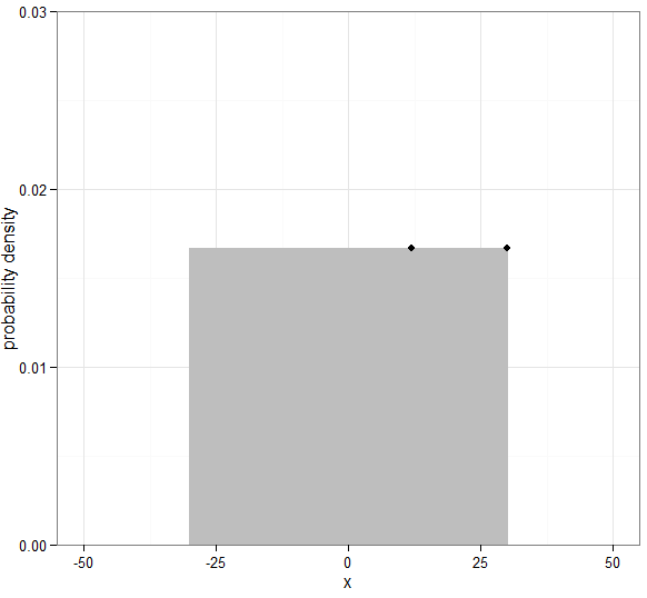
Try $a=30$
The PDF of the uniform distribution will be $\frac{1}{60} = 0.01\dot{6}$ for $x \in [-30, 30]$ and $0$ otherwise. The probability density of $x_1 = 12$ will be $\frac{1}{60}$, and so will be the probability density of $x_2=30$. The joint density will be $\frac{1}{60} \times \frac{1}{60} = \frac{1}{3600} = 0.0002\dot{7}$.

This is the best we can do! If we make the interval any narrow, $a=30$ will lie outside the support, and the likelihood will fall to zero. So the maximum likelihood occurs at $a=30$, and this is our maximum likelihood estimate.
A more useful approach
I hope you can now see conceptually why the maximum likelihood estimator is $a=30$. You can't play around with graphs so easily in your exam so you probably want a more general, algebraic solution. Finding a formula for the likelihood function basically requires you to find a formula for the joint density function for your sample, which I'll now assume to be of size $n$:
$$\vec{x}=(x_1, x_2, \dots, x_n)^T$$.
Now the joint density is zero if any of these lie outside the support $[-a, a]$. So for a non-zero joint density we need $-a \leq x_i \leq a$ for each $x_i$, which is the same as demanding each $|x_i| \leq a$. With a bit of thought, this in turn is equivalent to demanding $\max(|x_i|) \leq a$. So long as we are in the domain, the marginal density for each $x_i$ is independently $\frac{1}{2a}$ and the joint density will be the product of $n$ such marginal densities, so $f_a(\vec{x}) = \frac{1}{(2a)^n}$. Our final result is that:
$$\mathcal{L}(a|\vec{x})=f_a(\vec{x})=\begin{cases}
\frac{1}{(2a)^n} & a \geq \max(|x_i|) \\
0 & \text{otherwise}
\end{cases}$$
In your example, $n=2$ and $\max(|x_i|)=30$ so you are faced with the task of maximising:
$$\mathcal{L}(a|\vec{x})=f_a(\vec{x})=\begin{cases}
\frac{1}{(2a)^2} & a \geq 30 \\
0 & \text{otherwise}
\end{cases}$$
You may have been trained to think "aha, maximising requires calculus" and try differentiating and setting to zero, but don't do it! The function isn't continuous at the interesting part. Instead you should draw a graph of the likelihood for a range of values of $a$. You should be able to deduce $a=30$ quite quickly.
Code for plots
require(ggplot2)

#output is probability density
fxa <- function(x, a) {
  ifelse(abs(x)>a, 0, 1/a)
}

#output is a function, PDF for this value of a
fx <- function(a) {
  function(x) fxa(x, a)
}

plota <- function(a) {
  x.df <- data.frame(x=c(12, 30))
  x.df$density <- (fx(a))(x.df$x)
  ggplot(data.frame(x=c(-50, 50)), aes(x)) +
    coord_cartesian(ylim = c(0, 0.05)) +
    stat_function(geom="area", fun=fx(a), n=1e3, fill="grey") +
    geom_point(data=x.df, aes(x=x, y=density)) +
    theme_bw() + ylab("probability density")
}
The graphs are generated just by specifying a particular value of $a$, e.g. plota(25) for $a = 25$.

