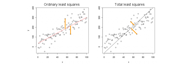
Ordinary least squares vs. total least squares
Let's first consider the simplest case of only one predictor (independent) variable $x$. For simplicity, let both $x$ and $y$ be centered, i.e. intercept is always zero. The difference between standard OLS regression and "orthogonal" TLS regression is clearly shown on this (adapted by me) figure from the most popular answer in the most popular thread on PCA:

OLS fits the equation $y=\beta x$ by minimizing squared distances between observed values $y$ and predicted values $\hat y$. TLS fits the same equation by minimizing squared distances between $(x,y)$ points and their projection on the line. In this simplest case TLS line is simply the first principal component of the 2D data. To find $\beta$, do PCA on $(x,y)$ points, i.e. construct the $2\times 2$ covariance matrix $\boldsymbol \Sigma$ and find its first eigenvector $\mathbf v = (v_x, v_y)$; then $\beta = v_y/v_x$.
In Matlab:
 v = pca([x y]);    //# x and y are centered column vectors
 beta = v(2,1)/v(1,1);
In R:
 v <- prcomp(cbind(x,y))$rotation
 beta <- v[2,1]/v[1,1]
By the way, this will yield correct slope even if $x$ and $y$ were not centered (because built-in PCA functions automatically perform centering). To recover the intercept, compute $\beta_0 = \bar y - \beta \bar x$.
OLS vs. TLS, multiple regression
Given a dependent variable $y$ and many independent variables $x_i$ (again, all centered for simplicity), regression fits an equation $$y= \beta_1 x_1 + \ldots + \beta_p x_p.$$ OLS does the fit by minimizing the squared errors between observed values of $y$ and predicted values $\hat y$. TLS does the fit by minimizing the squared distances between observed $(\mathbf x, y)\in\mathbb R^{p+1}$ points and the closest points on the regression plane/hyperplane.
Note that there is no "regression line" anymore! The equation above specifies a hyperplane: it's a 2D plane if there are two predictors, 3D hyperplane if there are three predictors, etc. So the solution above does not work: we cannot get the TLS solution by taking the first PC only (which is a line). Still, the solution can be easily obtained via PCA.
As before, PCA is performed on $(\mathbf x, y)$ points. This yields $p+1$ eigenvectors in columns of $\mathbf V$. The first $p$ eigenvectors define a $p$-dimensional hyperplane $\mathcal H$ that we need; the last (number $p+1$) eigenvector $\mathbf v_{p+1}$ is orthogonal to it. The question is how to transform the basis of $\mathcal H$ given by the first $p$ eigenvectors into the $\boldsymbol \beta$ coefficients.
Observe that if we set $x_i=0$ for all $i \ne k$ and only $x_k=1$, then $\hat y=\beta_k$, i.e. the vector $$(0,\ldots, 1, \ldots, \beta_k) \in \mathcal H$$ lies in the hyperplane $\mathcal H$. On the other hand, we know that $$\mathbf v_{p+1}=(v_1, \ldots, v_{p+1}) \:\bot\: \mathcal H$$ is orthogonal to it. I.e. their dot product must be zero: $$v_k + \beta_k v_{p+1}=0 \Rightarrow \beta_k = -v_k/v_{p+1}.$$
In Matlab:
 v = pca([X y]);    //# X is a centered n-times-p matrix, y is n-times-1 column vector
 beta = -v(1:end-1,end)/v(end,end);
In R:
 v <- prcomp(cbind(X,y))$rotation
 beta <- -v[-ncol(v),ncol(v)] / v[ncol(v),ncol(v)]
Again, this will yield correct slopes even if $x$ and $y$ were not centered (because built-in PCA functions automatically perform centering). To recover the intercept, compute $\beta_0 = \bar y - \bar {\mathbf x} \boldsymbol \beta$.
As a sanity check, notice that this solution coincides with the previous one in case of only a single predictor $x$. Indeed, then the $(x,y)$ space is 2D, and so, given that the first PCA eigenvector is orthogonal to the second (last) one, $v^{(1)}_y/v^{(1)}_x=-v^{(2)}_x/v^{(2)}_y$.
Closed form solution for TLS
Surprisingly, it turns out that there is a closed form equation for $\boldsymbol \beta$. The argument below is taken from Sabine van Huffel's book "The total least squares" (section 2.3.2).
Let $\mathbf X$ and $\mathbf y$ be the centered data matrices. The last PCA eigenvector $\mathbf v_{p+1}$ is an eigenvector of the covariance matrix of $[\mathbf X\: \mathbf y]$ with an eigenvalue $\sigma^2_{p+1}$. If it is an eigenvector, then so is $-\mathbf v_{p+1}/v_{p+1} = (\boldsymbol \beta\:\: -1)^\top$. Writing down the eigenvector equation:
$$\left(\begin{array}{c}\mathbf X^\top \mathbf X & \mathbf X^\top \mathbf y\\ \mathbf y^\top \mathbf X & \mathbf y^\top \mathbf y\end{array}\right) \left(\begin{array}{c}\boldsymbol \beta \\ -1\end{array}\right) = \sigma^2_{p+1}\left(\begin{array}{c}\boldsymbol \beta \\ -1\end{array}\right),$$
and computing the product on the left, we immediately get that $$\boldsymbol \beta_\mathrm{TLS} = (\mathbf X^\top \mathbf X - \sigma^2_{p+1}\mathbf I)^{-1} \mathbf X^\top \mathbf y,$$ which strongly reminds the familiar OLS expression $$\boldsymbol \beta_\mathrm{OLS} = (\mathbf X^\top \mathbf X)^{-1} \mathbf X^\top \mathbf y.$$
Multivariate multiple regression
The same formula can be generalized to the multivariate case, but even to define what multivariate TLS does, would require some algebra. See Wikipedia on TLS. Multivariate OLS regression is equivalent to a bunch of univariate OLS regressions for each dependent variable, but in the TLS case it is not so.

