289
$\begingroup$

I was skimming through some lecture notes by Cosma Shalizi (in particular, section 2.1.1 of the second lecture), and was reminded that you can get very low $R^2$ even when you have a completely linear model.

To paraphrase Shalizi's example: suppose you have a model $Y = aX + \epsilon$, where $a$ is known. Then $\newcommand{\Var}{\mathrm{Var}}\Var[Y] = a^2 \Var[x] + \Var[\epsilon]$ and the amount of explained variance is $a^2 \Var[X]$, so $R^2 = \frac{a^2 \Var[x]}{a^2 \Var[X] + \Var[\epsilon]}$. This goes to 0 as $\Var[X] \rightarrow 0$ and to 1 as $\Var[X] \rightarrow \infty$.

Conversely, you can get high $R^2$ even when your model is noticeably non-linear. (Anyone have a good example offhand?)

So when is $R^2$ a useful statistic, and when should it be ignored?

$\endgroup$
10
  • 5
    $\begingroup$ Please note the related comment thread in another recent question $\endgroup$
    – whuber
    Commented Jul 20, 2011 at 20:47
  • 42
    $\begingroup$ I have nothing statistical to add to the excellent answers given (esp. the one by @whuber) but I think the right answer is "R-squared: Useful and dangerous". Like pretty much any statistic. $\endgroup$
    – Peter Flom
    Commented Jul 21, 2011 at 10:47
  • 39
    $\begingroup$ The answer to this question is: "Yes" $\endgroup$
    – Fomite
    Commented Apr 23, 2012 at 20:52
  • 1
    $\begingroup$ See stats.stackexchange.com/a/265924/99274 for yet another answer. $\endgroup$
    – Carl
    Commented Mar 8, 2017 at 2:16
  • 3
    $\begingroup$ just a thought - if $Var(X)\approx 0$ then $aX\approx const$ which means the model is close to $Y=const+\epsilon$. this means $R^2\approx 0$ is a good thing! $\endgroup$ Commented May 21, 2019 at 6:34

6 Answers 6

326
$\begingroup$

To address the first question, consider the model

$$Y = X + \sin(X) + \varepsilon$$

with iid $\varepsilon$ of mean zero and finite variance. As the range of $X$ (thought of as fixed or random) increases, $R^2$ goes to 1. Nevertheless, if the variance of $\varepsilon$ is small (around 1 or less), the data are "noticeably non-linear." In the plots, $var(\varepsilon)=1$.
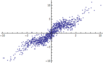
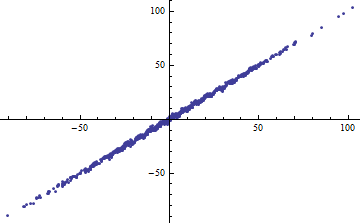
Short range of X

Wider range of X

Incidentally, an easy way to get a small $R^2$ is to slice the independent variables into narrow ranges. The regression (using exactly the same model) within each range will have a low $R^2$ even when the full regression based on all the data has a high $R^2$. Contemplating this situation is an informative exercise and good preparation for the second question.

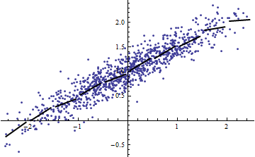
Both the following plots use the same data. The $R^2$ for the full regression is 0.86. The $R^2$ for the slices (of width 1/2 from -5/2 to 5/2) are .16, .18, .07, .14, .08, .17, .20, .12, .01, .00, reading left to right. If anything, the fits get better in the sliced situation because the 10 separate lines can more closely conform to the data within their narrow ranges. Although the $R^2$ for all the slices are far below the full $R^2$, neither the strength of the relationship, the linearity, nor indeed any aspect of the data (except the range of $X$ used for the regression) has changed.
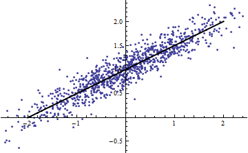
Point cloud with full regression

Sliced point cloud with 10 regressions

(One might object that this slicing procedure changes the distribution of $X$. That is true, but it nevertheless corresponds with the most common use of $R^2$ in fixed-effects modeling and reveals the degree to which $R^2$ is telling us about the variance of $X$ in the random-effects situation. In particular, when $X$ is constrained to vary within a smaller interval of its natural range, $R^2$ will usually drop.)

The basic problem with $R^2$ is that it depends on too many things (even when adjusted in multiple regression), but most especially on the variance of the independent variables and the variance of the residuals. Normally it tells us nothing about "linearity" or "strength of relationship" or even "goodness of fit" for comparing a sequence of models.

Most of the time you can find a better statistic than $R^2$. For model selection you can look to AIC and BIC; for expressing the adequacy of a model, look at the variance of the residuals.

This brings us finally to the second question. One situation in which $R^2$ might have some use is when the independent variables are set to standard values, essentially controlling for the effect of their variance. Then $1 - R^2$ is really a proxy for the variance of the residuals, suitably standardized.

$\endgroup$
18
  • 35
    $\begingroup$ What an amazingly thorough and responsive answer by @whuber $\endgroup$
    – Peter Flom
    Commented Jul 21, 2011 at 10:40
  • 8
    $\begingroup$ @dr My critique applies perfectly to adjusted $R^2$. The only cases where there's much of a difference between $R^2$ and the adjusted $R^2$ are when you are using loads of parameters compared to the data. In the slicing example there were almost 1,000 data points and the slicing added only 18 parameters; the adjustments to $R^2$ wouldn't even affect the second decimal place, except possibly in the end segments where there were only a few dozen data points: and it would lower them, actually strengthening the argument. $\endgroup$
    – whuber
    Commented Jul 22, 2011 at 14:01
  • 6
    $\begingroup$ The answer to the question in your first comment ought to depend on your objective and there are several ways to interpret "testing for a linear relationship." One is, you want to test whether the coefficient is nonzero. Another is, you want to know whether there is evidence of nonlinearity. $R^2$ (by itself) isn't terribly useful for either, although we know that a high $R^2$ with plenty of data means their scatterplot looks roughly linear--like my second one or like @macro's example. For each objective there is an appropriate test and its associated p-value. $\endgroup$
    – whuber
    Commented Jul 22, 2011 at 16:41
  • 4
    $\begingroup$ For your second question we ought to wonder what might be meant by "best" linear fit. One candidate would be any fit that minimizes the residual sum of squares. You could safely use $R^2$ as a proxy for this, but why not examine the (adjusted) root mean square error itself? It's a more useful statistic. $\endgroup$
    – whuber
    Commented Jul 22, 2011 at 16:44
  • 1
    $\begingroup$ (+1) It was hard for me to explain why there is a huge difference in $R^2$ in fixed effects models as compared to pulled regression or random effects, now I know how to explain this part (the answer, in my opinion, worths +100 only for this part). $\endgroup$ Commented Aug 22, 2011 at 9:07
53
$\begingroup$

Your example only applies when the variable $\newcommand{\Var}{\mathrm{Var}}X$ should be in the model. It certainly doesn't apply when one uses the usual least squares estimates. To see this, note that if we estimate $a$ by least squares in your example, we get:

$$\hat{a}=\frac{\frac{1}{N}\sum_{i=1}^{N}X_{i}Y_{i}}{\frac{1}{N}\sum_{i=1}^{N}X_{i}^{2}}=\frac{\frac{1}{N}\sum_{i=1}^{N}X_{i}Y_{i}}{s_{X}^{2}+\overline{X}^{2}}$$ Where $s_{X}^2=\frac{1}{N}\sum_{i=1}^{N}(X_{i}-\overline{X})^{2}$ is the (sample) variance of $X$ and $\overline{X}=\frac{1}{N}\sum_{i=1}^{N}X_{i}$ is the (sample) mean of $X$

$$\hat{a}^{2}\Var[X]=\hat{a}^{2}s_{X}^{2}=\frac{\left(\frac{1}{N}\sum_{i=1}^{N}X_{i}Y_{i}\right)^2}{s_{X}^2}\left(\frac{s_{X}^{2}}{s_{X}^{2}+\overline{X}^{2}}\right)^2$$

Now the second term is always less than $1$ (equal to $1$ in the limit) so we get an upper bound for the contribution to $R^2$ from the variable $X$:

$$\hat{a}^{2}\Var[X]\leq \frac{\left(\frac{1}{N}\sum_{i=1}^{N}X_{i}Y_{i}\right)^2}{s_{X}^2}$$

And so unless $\left(\frac{1}{N}\sum_{i=1}^{N}X_{i}Y_{i}\right)^2\to\infty$ as well, we will actually see $R^2\to 0$ as $s_{X}^{2}\to\infty$ (because the numerator goes to zero, but denominator goes into $\Var[\epsilon]>0$). Additionally, we may get $R^2$ converging to something in between $0$ and $1$ depending on how quickly the two terms diverge. Now the above term will generally diverge faster than $s_{X}^2$ if $X$ should be in the model, and slower if $X$ shouldn't be in the model. In both case $R^2$ goes in the right directions.

And also note that for any finite data set (i.e. a real one) we can never have $R^2=1$ unless all the errors are exactly zero. This basically indicates that $R^2$ is a relative measure, rather than an absolute one. For unless $R^2$ is actually equal to $1$, we can always find a better fitting model. This is probably the "dangerous" aspect of $R^2$ in that because it is scaled to be between $0$ and $1$ it seems like we can interpet it in an absolute sense.

It is probably more useful to look at how quickly $R^2$ drops as you add variables into the model. And last, but not least, it should never be ignored in variable selection, as $R^2$ is effectively a sufficient statistic for variable selection - it contains all the information on variable selection that is in the data. The only thing that is needed is to choose the drop in $R^2$ which corresponds to "fitting the errors" - which usually depends on the sample size and the number of variables.

$\endgroup$
1
  • 5
    $\begingroup$ +1 Lots of nice points. The calculations add quantitative insights to the previous replies. $\endgroup$
    – whuber
    Commented Aug 23, 2011 at 16:44
31
$\begingroup$

If I can add an example of when $R^2$ is dangerous. Many years ago I was working on some biometric data and being young and foolish I was delighted when I found some statistically significant $R^2$ values for my fancy regressions which I had constructed using stepwise functions. It was only afterwards looking back after my presentation to a large international audience did I realize that given the massive variance of the data - combined with the possible poor representation of the sample with respect to the population, an $R^2$ of 0.02 was utterly meaningless even if it was "statistically significant"...

Those working with statistics need to understand the data!

$\endgroup$
6
  • 21
    $\begingroup$ No statistic is dangerous if you understand what it means. Sean's example has nothing special to do with R square it is the general problem of being enamored with statistical significance. When we do statistical testing in practice we are only interested in meaningful differences. Two populations never have identical distributions. If they are close to equal we don't care. With very large sample sizes we can detect small unimportant differences. That is why in my medical research consulting I emphasize the difference between clinical and statistical significance. $\endgroup$ Commented May 6, 2012 at 1:16
  • 11
    $\begingroup$ Initially my clients often thin that statistical significance is the goal of the research. They need to be shown that it is not the case. $\endgroup$ Commented May 6, 2012 at 1:16
  • 3
    $\begingroup$ A statistically significant $R^2$ at 0.02 simply means that you had sufficient data to claim that $R^2$ is not 0. But it is close to 0. So there is very little of a relationship between the independent variables and dependent variable. $\endgroup$ Commented Aug 22, 2019 at 23:47
  • 3
    $\begingroup$ Absolutely agree Michael. A little knowledge of statistics can be dangerous! :) Based on that insight many years ago, I worked hard not to repeat that daft mistake by doing a lot of study to better understand what statistics really mean. A masters degree and a PhD in statistics and I still think I have a long way to go with my studies! $\endgroup$
    – Sean
    Commented Aug 24, 2019 at 6:22
  • $\begingroup$ Thank you Sean. I appreciate your comments and humility. $\endgroup$ Commented Aug 24, 2019 at 17:00
18
$\begingroup$

When you have a single predictor $R^{2}$ is exactly interpreted as the proportion of variation in $Y$ that can be explained by the linear relationship with $X$. This interpretation must be kept in mind when looking at the value of $R^2$.

You can get a large $R^2$ from a non-linear relationship only when the relationship is close to linear. For example, suppose $Y = e^{X} + \varepsilon$ where $X \sim {\rm Uniform}(2,3)$ and $\varepsilon \sim N(0,1)$. If you do the calculation of

$$ R^{2} = {\rm cor}(X, e^{X} + \varepsilon)^{2} $$

you will find it to be around $.914$ (I only approximated this by simulation) despite that the relationship is clearly not linear. The reason is that $e^{X}$ looks an awful lot like a linear function over the interval $(2,3)$.

$\endgroup$
4
  • 1
    $\begingroup$ To the remarks below by Erik and Macro I don't think anyone has it out for me and it is probably better to have one combined answer instead of three separate ones but why does it matter to the point that so much discussion centers around how you write things and where you write it instead of fcusing on what is said? $\endgroup$ Commented May 6, 2012 at 4:13
  • 8
    $\begingroup$ @MichaelChernick, I don't think there is "so much" discussion about how one writes things. The guidelines we've tried to help you with are more along the lines of "if everyone did that, this site would be very disorganized and hard to follow". It may seem like there is a lot of discussion about these things, but that's probably just because you've been a very active participant since you joined, which is great, since you clearly bring a lot to the table. If you want to talk more about this, consider starting a thread on meta rather than a comment discussion under my unrelated answer :) $\endgroup$
    – Macro
    Commented May 6, 2012 at 4:40
  • $\begingroup$ what does happed if one widers support of uniform distribution in your example ? $\endgroup$
    – Qbik
    Commented Jan 22, 2015 at 12:31
  • 2
    $\begingroup$ As I have gained experience on this site I have to agree with Macro that it is important to be concise and consolidate. $\endgroup$ Commented Aug 24, 2019 at 16:59
17
$\begingroup$

One situation you would want to avoid $R^2$ is multiple regression, where adding irrelevant predictor variables to the model can in some cases increase $R^2$. This can be addressed by using the adjusted $R^2$ value instead, calculated as

$\bar{R}^2 = 1 - (1-R^2)\frac{n-1}{n-p-1}$ where $n$ is the number of data samples, and $p$ is the number of regressors not counting the constant term.

$\endgroup$
1
  • 26
    $\begingroup$ Note that adding irrelevant variables is guaranteed to increase $R^2$ (not just in "some cases") unless those variables are completely collinear with the existing variables. $\endgroup$
    – whuber
    Commented Jan 9, 2012 at 18:57
9
$\begingroup$
  1. A good example for high $R^2$ with a nonlinear function is the quadratic function $y=x^2$ restricted to the interval $[0,1]$. With 0 noise it will not have an $R^2$ square of 1 if you have 3 or more points since they will not fit perfectly on a straight line. But if the design points are scattered uniformly on the $[0, 1]$ the $R^2$ you get will be high perhaps surprisingly so. This may not be the case if you have a lot of points near 0 and a lot near 1 with little or nothing in the middle.

  2. $R^2$ will be poor in the perfect linear case if the noise term has a large variance. So you can take the model $Y= x + \epsilon$ which is technically a perfect linear model but let the variance in e tend to infinity and you will have $R^2$ going to 0. Inspite of its deficiencies R square does measure the percentage of variance explained by the data and so it does measure goodness of fit. A high $R^2$ means a good fit but we still have to be careful about the good fit being caused by too many parameters for the size of the data set that we have.

  3. In the multiple regression situation there is the overfitting problem. Add variables and $R^2$ will always increase. The adjusted $R^2$ remedies this somewhat as it takes account of the number of parameters being estimated.

$\endgroup$
0

Your Answer

By clicking “Post Your Answer”, you agree to our terms of service and acknowledge you have read our privacy policy.

Not the answer you're looking for? Browse other questions tagged or ask your own question.