K-means++ algorithm

Question

I try to implement k-means++, but I'm not sure how it works. I have the following dataset:

(7,1), (3,4), (1,5), (5,8), (1,3), (7,8), (8,2), (5,9), (8,0)

From the wikipedia:

• Step 1: Choose one center uniformly at random from among the data points.

  let's say the first centroid is 8,0

• Step 2: For each data point x, compute D(x), the distance between x and the nearest center that has already been chosen.

  I calculate all each point's distance to tht point nr.9 (8,0)

  • 1 (7,1) distance = (8-7)^2 + (0-1)^2 = (1)^2 + (-1)^2 = 1 + 1 = 2
  • 2 (3,4) distance = (8-3)^2 + (0-4)^2 = (5)^2 + (-4)^2 = 25 + 16 = 41
  • 3 (1,5) distance = (8-1)^2 + (0-5)^2 = (7)^2 + (-5)^2 = 49 + 25 = 74
  • 4 (5,8) distance = (8-5)^2 + (0-8)^2 = (3)^2 + (-8)^2 = 9 + 64 = 73
  • 5 (1,3) distance = (8-1)^2 + (0-3)^2 = (7)^2 + (-3)^2 = 49 + 9 = 58
  • 6 (7,8) distance = (8-7)^2 + (0-8)^2 = (1)^2 + (-8)^2 = 1 + 64 = 65
  • 7 (8,2) distance = (8-8)^2 + (0-2)^2 = (0)^2 + (-2)^2 = 0 + 4 = 4
  • 8 (5,9) distance = (8-5)^2 + (0-9)^2 = (3)^2 + (-9)^2 = 9 + 81 = 90

• Step 3: Choose one new data point at random as a new center, using a weighted probability distribution where a point x is chosen with probability proportional to $D(x)^2$.

• Step 4: Repeat Steps 2 and 3 until k centers have been chosen.

Could someone explain in detail how to calculate the 3rd step?

Answer 1

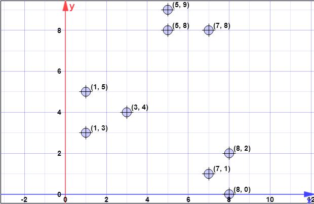
Here is my code, in Mathematica:

data = {{7, 1}, {3, 4}, {1, 5}, {5, 8}, {1, 3}, {7, 8}, {8, 2}, {5, 9}, {8, 0}};
centers = {};
RelativeWeights = Table[1/Length[data], {Length[data]}];
Table[
  centers = 
   Union[RandomChoice[RelativeWeights -> data , 1], centers];
  data = Complement[data, centers];
  RelativeWeights = 
   Normalize@(EuclideanDistance[#1[[1]], Nearest[centers, #1]]^2 & /@ 
      data);
  {centers, data},
  {3}] // TableForm

Here is how it works:

• The data set is defined
• We start with no centers
• The RelativeWeights (which govern the probability that a current data point will be selected to be a new, additional center) are initially set to be equal for all the current data points. Incidentally, Length[data] is merely the number of elements in the list called data.
• Now, Table is an iterator (like a DO statement), which here runs through the algorithm k times, where I set k = 3
• RandomChoice chooses 1 member of the set data according to the RelativeWeights, and adds this chosen center to the list of centers, and removes it from data
• The RelativeWeights are updated by taking each element in data in turn, and finding the Nearest element in the current list of centers, then computing its EuclideanDistance (squared) to that point. Your problem stated "distance," but the Wikipedia page for the algorithm stated distance squared. (The weights are then normalized to 1, to make a true discrete distribution, but this step is not needed as Mathematica automatically normalizes in this case)
• Then we store the current list of centers and data.

$\left( \begin{array}{cc} \left( \begin{array}{cc} 1 & 5 \\ \end{array} \right) & \left( \begin{array}{cc} 1 & 3 \\ 3 & 4 \\ 5 & 8 \\ 5 & 9 \\ 7 & 1 \\ 7 & 8 \\ 8 & 0 \\ 8 & 2 \\ \end{array} \right) \\ \left( \begin{array}{cc} 1 & 5 \\ 7 & 8 \\ \end{array} \right) & \left( \begin{array}{cc} 1 & 3 \\ 3 & 4 \\ 5 & 8 \\ 5 & 9 \\ 7 & 1 \\ 8 & 0 \\ 8 & 2 \\ \end{array} \right) \\ \left( \begin{array}{cc} 1 & 3 \\ 1 & 5 \\ 7 & 8 \\ \end{array} \right) & \left( \begin{array}{cc} 3 & 4 \\ 5 & 8 \\ 5 & 9 \\ 7 & 1 \\ 8 & 0 \\ 8 & 2 \\ \end{array} \right) \\ \end{array} \right)$

As you can see, the first data point chosen to be a center was (1,5), and the other points remained. Next, the point (7,8) was chosen and added to the list of centers, and so on.

The precise mathematics behind the third step is straightforward: For each point in data, find its distance to the nearest center, $d_i$. If there are $r$ elements currently in data, then you have $r$ distances--one for each point. The overall goal of kmeans++ is to choose new points from data that are FAR from existing centers, so we want to increase the probability of being chosen for points in data that are far from any center.

We do this as follows: We sum up all the $r$ distances to get $s_{tot}$:

$s_{tot} = \sum_{i=1}^r d_i$ .

For each point in data, we compute its distance divided by $s_{tot}$ and set that to the probability that point will be chosen as a new, additional, center:

$p_i = d_i/s_{tot}$.

Notice that the sum of all $r$ probabilities will add up to 1.0, as is required for a true probability.

Now, we want to choose a new point in data proportional to its probability $p_i$. Because of how we computed $p_i$, points far from any center (i.e., with large $p_i$) are more likely to be chosen than points with small $p_i$---just as the algorithm wants.

You can implement such a probability proportional selection by dividing up the unit interval ($0 \rightarrow 1$) by segments of length $p_i$ and uniformly choosing a value between 0 and 1 and finding which interval (i.e., which point) the random selected value lands in.

This is a full, precise mathematical explanation of kmeans++. I cannot see that there is anything more needed to describe it, especially since the working code is present for all.

Answer 2

For step 3,

Choose one new data point at random as a new center, using a weighted probability distribution where a point x is chosen with probability proportional to $D(x)^2$.

Compute all the $D(x)^2$ values and convert them to an array of cumulative sums. That way each item is represented by a range proportional to its value. Then pick a uniform random number in that range and see which item it corresponds to (using a binary search).

For instance, you have:

D(x)^2 = [2, 41, 74, 73, 58, 65, 4, 90]
cumulative D(x)^2 = [2, 43, 117, 190, 248, 313, 317, 407]

So pick a random number from [0, 407). Say you pick 123.45. It falls in the range [117, 190) which corresponds to the 4th item.