Regression trees to model rates

Question

I am performing a predictive modeling application where I have to predict claims. If I had used classical GLMs, I would have used a poisson glm using log exposure as offset, assuming therefore $$\text{claims} = \text{exposure} \cdot \exp \left( x^T \beta \right),$$ assuming that claims are proportional to the exposure and therefore allowing for covariate dependency. I want to use ctree or rpart or other tree based approaches. Is it possible to handle prior offset in such models in some way?

Answer 1

One way would be to adopt a formal model-based tree. The glmtree() function in the partykit package implements the general MOB algorithm for model-based recursive partitioning (Zeileis et al. 2008, Journal of Computational and Graphical Statistics, 17(2), 492-514). This supports Poisson responses and also allows for the inclusion of offsets. Furthermore, additional regressors could be included in each of the terminal nodes.

Consider the following simple artificial example:

set.seed(1)
d <- data.frame(
  x1 = runif(500),
  x2 = runif(500),
  exposure = runif(500, 1, 10)
)
d$claims <- rpois(500, lambda = exp(d$x1 > 0.5 & d$x2 > 0.5) * d$exposure)

This uses two simple partitioning variables (x1 and x2) and an exposure variable. The response is Poisson-distributed with offset log(exposure) and mean 1 = exp(0) except for the case when both x1 > 0.5 & x2 > 0.5 where the mean is exp(1)

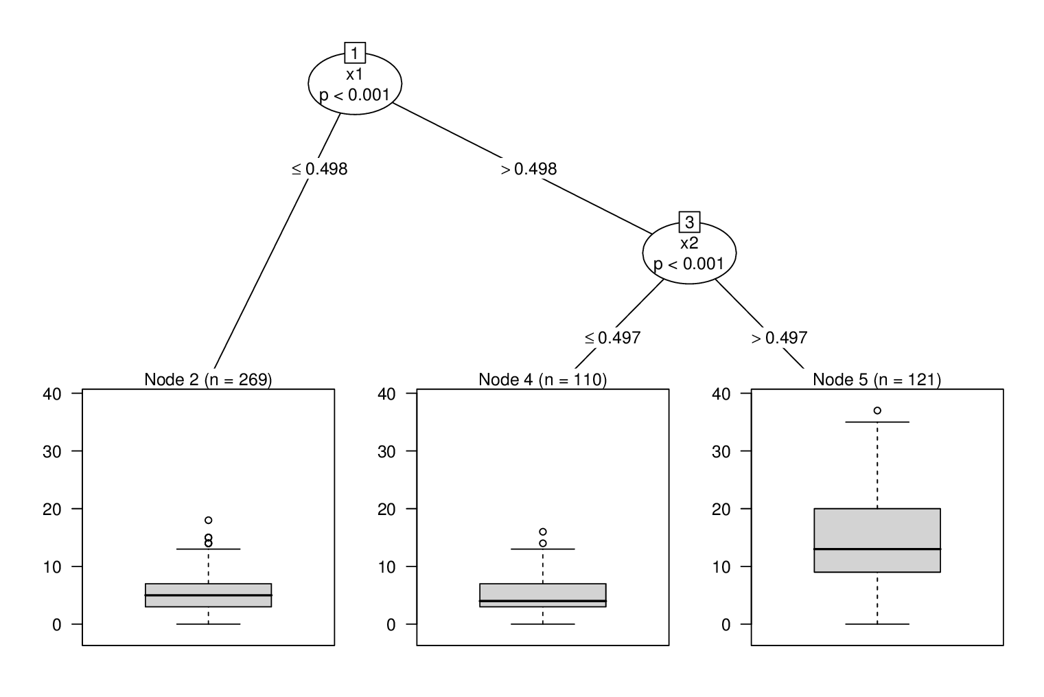
Then glmtree() can fit a Poisson GLM-based tree for claims with offset(log(exposure)) and partitioning variables x1 + x2.

m <- glmtree(claims ~ offset(log(exposure)) | x1 + x2,
  data = d, family = poisson)
plot(as.constparty(m))

This captures the true tree structure (which is admittedly easy to find here) and correctly estimates the intercepts (with the default log-link):

coef(m)

##            2            4            5 
## -0.047934373 -0.005690107  1.050569309 

You can also obtain more detailed information about each fitted GLM in the nodes of the tree, e.g., for the last node:

summary(m, node = 5)

## Call:
## glm(formula = claims ~ offset(log(exposure)))
## 
## Deviance Residuals: 
##      Min        1Q    Median        3Q       Max  
## -3.13527  -0.66977  -0.04251   0.56984   2.13581  
## 
## Coefficients:
##             Estimate Std. Error z value Pr(>|z|)    
## (Intercept)  1.05057    0.02375   44.24   <2e-16 ***
## ---
## Signif. codes:  0 '***' 0.001 '**' 0.01 '*' 0.05 '.' 0.1 ' ' 1
## 
## (Dispersion parameter for poisson family taken to be 1)
## 
##     Null deviance: 630.95  on 120  degrees of freedom
## Residual deviance: 113.36  on 120  degrees of freedom
## AIC: 635.89
## 
## Number of Fisher Scoring iterations: 4

More details and references are provided in vignette("mob", package = "partykit").