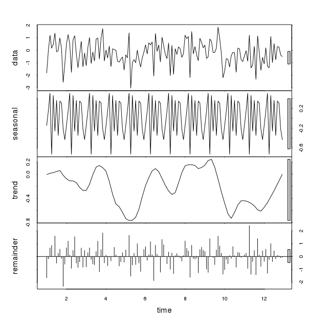
Loess decomposition is intended to smooth the series by applying averages to the data so that it collapses into components, e.g. the trend or seasonal, that are interesting for the analysis of the data. But this methodology is not intended to do a formal test for the presence of seasonality.
Although in your example stl returns a smoothed pattern of seasonal periodicity, this pattern is not relevant to explain the dynamics of the series. In order to see that, we can compare the variance of each component with respect to the variance of the original series.
set.seed(123)
x <- ts(rnorm(144, sd=1), frequency=12)
a <- stl(x, s.window="periodic")
apply(a$time.series, 2, var) / var(x)
#   seasonal      trend  remainder
# 0.07080362 0.07487838 0.81647852
We can see that it is the remainder what explains most of the variance in the data (as we would expect for a white noise process).
If we take a series with seasonality, the relative variance of the seasonal component is much more relevant (although we don't have a straightforward way to test it since loess is not parametric).
y <- diff(log(AirPassengers))
b <- stl(y, s.window="periodic")
apply(b$time.series, 2, var) / var(y)
#    seasonal       trend   remainder
# 0.875463620 0.001959407 0.117832537
The relative variances indicate that seasonality is the main component explaining the dynamics of the series.
A careless look at the plot from stl can be deceptive. The nice pattern returned by stl may make us think that a relevant seasonal pattern can be identified in the data, but a closer look may reveal that it's not actually the case. If the purpose is to decide on the presence of seasonality, loess decomposition can be useful as a preliminary view but it should be complemented with other tools.


