Generate two samples of correlated data from a standard normal random distribution following a predetermined correlation.
As an example, let's pick a correlation r = 0.7, and code a correlation matrix such as:
(C <- matrix(c(1,0.7,0.7,1), nrow = 2))
     [,1] [,2]
[1,]  1.0  0.7
[2,]  0.7  1.0
We can use mvtnorm to generate now these two samples as a bivariate random vector:
set.seed(0)
SN <- rmvnorm(mean = c(0,0), sig = C, n = 1e5) resulting in two vector components distributed as ~ $N(0, 1)$ and with a cor(SN[,1],SN[,2])= 0.6996197 ~ 0.7. Both components can be extricated as follows:
X1 <- SN[,1]; X2 <- SN[,2]
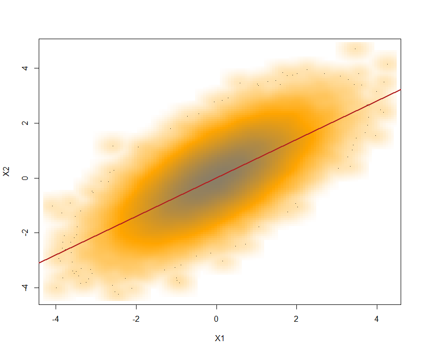
Here's the plot with the overlapping regression line:

Use the Probability Integral Transform here to obtain a bivariate random vector with marginal distributions ~ $U(0, 1)$ and the same correlation:
U <- pnorm(SN) - so we are feeding into pnorm the SN vector to find $erf(SN)$ (or $\Phi(SN)$). In the process, we preserve the cor(U[,1], U[,2]) = 0.6816123 ~ 0.7 .
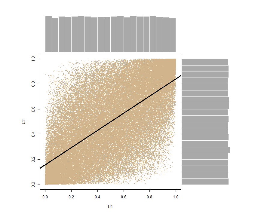
Again we can decompose the vector U1 <- U[,1]; U2 <- U[,2] and produce a scatterplot with marginal distributions at the edges, clearly showing their uniform nature:

Apply the inverse transform sampling method here to finally obtain the bivector of equally correlated points belonging to whichever distribution family we set out to reproduce.
From here we can just generate two vectors distributed normally and with equal or different variances. For instance: Y1 <- qnorm(U1, mean = 8,sd = 10) and Y2 <- qnorm(U2, mean = -5, sd = 4), which will maintain the desired correlation, cor(Y1,Y2) = 0.6996197 ~ 0.7.
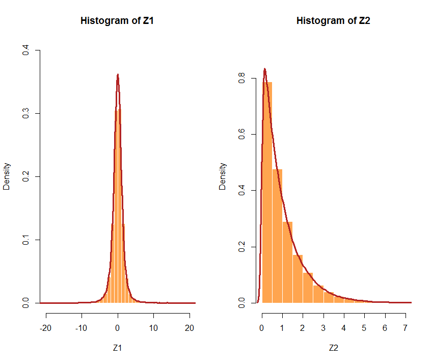
Or opt for different distributions. If the distributions chosen are very dissimilar, the correlation may not be as precise. For instance, let's get U1 to follow a $t$ distribution with 3 d.f., and U2 an exponential with a $\lambda$=1: Z1 <- qt(U1, df = 3) and Z2 <- qexp(U2, rate = 1) The cor(Z1,Z2) [1] 0.5941299 < 0.7. Here are the respective histograms:

Here is an example of code for the entire process and normal marginals:
Cor_samples <- function(r, n, mean1, mean2, sd1, sd2){
C <- matrix(c(1,r,r,1), nrow = 2)
require(mvtnorm)
SN <- rmvnorm(mean = c(0,0), sig = C, n = n)
U <- pnorm(SN)
U1 <- U[,1]
U2 <- U[,2]

 Y1 <<- qnorm(U1, mean = mean1,sd = sd1)
 Y2 <<- qnorm(U2, mean = mean2,sd = sd2)

sample_measures <<- as.data.frame(c(mean(Y1), mean(Y2), sd(Y1), sd(Y2), cor(Y1,Y2)), names<-c("mean Y1", "mean Y2", "SD Y1", "SD Y2", "Cor(Y1,Y2)"))
sample_measures
}
For comparison, I've put together a function based on the Cholesky decomposition:
Cholesky_samples <- function(r, n, mean1, mean2, sd1, sd2){
C <- matrix(c(1,r,r,1), nrow = 2)
L <- chol(C)
X1 <- rnorm(n)
X2 <- rnorm(n)
X <- rbind(X1,X2)

Y <- t(L)%*%X
Y1 <- Y[1,]
Y2 <- Y[2,]

N_1 <<- Y[1,] * sd1 + mean1
N_2 <<- Y[2,] * sd2 + mean2

sample_measures <<- as.data.frame(c(mean(N_1), mean(N_2), sd(N_1), sd(N_2), cor(N_1, N_2)),
                  names<-c("mean N_1", "mean N_2", "SD N_1", "SD N_2","cor(N_1,N_2)"))
sample_measures
}
Trying both methods to generate correlated (say, $r=0.7$) samples distributed ~ $N(97,23)$ and $N(32,8)$ we get, setting set.seed(99):
Using the Uniform:
cor_samples(0.7, 1000, 97, 32, 23, 8)
           c(mean(Y1), mean(Y2), sd(Y1), sd(Y2), cor(Y1, Y2))
mean Y1                                            96.5298821
mean Y2                                            32.1548306
SD Y1                                              22.8669448
SD Y2                                               8.1150780
cor(Y1,Y2)                                          0.7061308
and Using the Cholesky:
Cholesky_samples(0.7, 1000, 97, 32, 23, 8)
             c(mean(N_1), mean(N_2), sd(N_1), sd(N_2), cor(N_1, N_2))
mean N_1                                                   96.4457504
mean N_2                                                   31.9979675
SD N_1                                                     23.5255419
SD N_2                                                      8.1459100
cor(N_1,N_2)                                                0.7282176

