I've been led to believe (see here and here) that Mahalanobis distance is the same as the Euclidean distance on the PCA-rotated data. In other words, taking multivariate normal data $X$, the Mahalanobis distance of all of the $x$'s from any given point (say $\mathbf{0}$) should be the same as the Euclidean distance of the entries of $X^{rot}$ from $\mathbf{0}$, where $X^{rot}$ is the product of the data and the PCA rotation matrix.
1. Is this true?
My code below is suggesting to me that it is not. In particular, it looks like the variance of the Mahalanobis distance around the PCA-Euclidean distance is increasing in the magnitude of the PCA-Euclidean distance. Is this a coding error, or a feature of the universe? Does it have to do with imprecision in an estimate of something? Something that gets squared?
N=1000
cr = runif(1,min=-1,max=1)
A = matrix(c(1,cr,cr,1),2)
e<-mvrnorm(n = N,rep(0,2),A)
mx = apply(e, 2, mean)
sx = apply(e, 2, sd)
e = t(apply(e,1,function(X){(X-mx)/sx}))
plot(e[,1],e[,2])
dum<-rep(0,2)
md = mahalanobis(e,dum,cov(e))

pc = prcomp(e,center=F,scale=F)
d<-as.matrix(dist(rbind(dum,pc$x),method='euclidean',diag=F))
d<-d[1,2:ncol(d)]
plot(d,md^.5)
abline(0,1)
2. If the answer to the above is true, can one use the PCA-rotated Euclidean distance as a stand-in for the Mahalanobis distance when $p>n$?
If not, is there a similar metric that captures multivariate distance, scaled by correlation, and for which distributional results exist to allow the calculation of the probability of an observation?
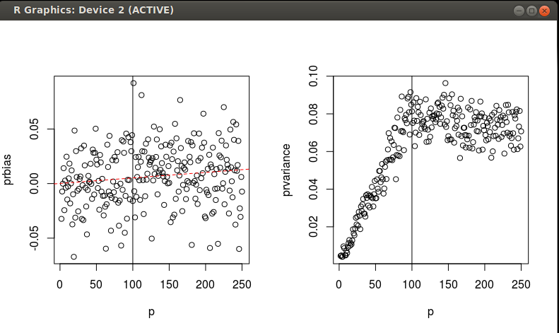
EDIT I've run a few simulations to investigate the equivalence of MD and SED on scaled/rotated data over a gradient of n and p. As I mentioned previously, I'm interested in the probability of an observation. I am hoping to find a good way to get the probability of an observation being part of a multivariate normal distribution, but for which I've got $n<p$ data to estimate the distribution. See the code below. It looks like the PCA-scaled/rotated SED is slightly biased estimator of the MD, with a fair amount of variance that seems to stop increasing when $p=N$.
f = function(N=1000,n,p){
  a = runif(p^2,-1,1)
  a = matrix(a,p)
  S = t(a)%*%a
  x = mvrnorm(N,rep(0,p),S)
  mx = apply(x, 2, mean)
  sx = apply(x, 2, sd)
  x = t(apply(x,1,function(X){(X-mx)/sx}))
  Ss = solve(cov(x))
  x = x[sample(1:N,n,replace=F),]
  md = mahalanobis(x,rep(0,p),Ss,inverted=T)
  prMD<-pchisq(md,df = p)
  pc = prcomp(x,center=F,scale=F)
  d<-mahalanobis(scale(pc$x),rep(0,ncol(pc$x)),diag(rep(1,ncol(pc$x))))
  prPCA<-pchisq(d,df = min(p,n))#N is the number of PCs where N<P
  return(data.frame(prbias = as.numeric(mean(prMD - prPCA)), prvariance = as.numeric(mean((prMD - prPCA)^2))))
}

grid = data.frame(n=100,p=2:200)
grid$prvariance <-grid$prbias <-NA

for (i in 1:nrow(grid)){
    o = f(n=grid[i,]$n,p=grid[i,]$p)
    grid[i,3:4]<-o
}

par(mfrow=c(1,2))
with(grid, plot(p,prbias))
abline(v=100)
m = lm(prbias~p,data=grid)
abline(m,col='red',lty=2)
with(grid, plot(p,prvariance))
abline(v=100)
Two questions: 1. Any criticism of what I'm finding in these simulations? 2. Can anyone formalize what I'm finding with an analytical expression for the bias and the variance as functions of n and p? I'd accept an answer that does this.


1/eigenvalueof the component. (And same hold also when we speak about distances between points and centroid, instead of point-point distances) This weighting is what compensates for the differences between Mahalanobis and Euclidean which I have touched in my comment. $\endgroup$Mahalanobis singularwhich might yield answers to your second question $\endgroup$