Markov Chain Monte Carlo (MCMC) with transformed data

Question

I want to obtain an estimate of a parameter $\Theta$ in a model for a random variable $X$ dependent on $\Theta$ with known but complicated likelihood $L(\Theta|X) = p(X|\Theta)$. $X$ is not directly observable, but I can observe transformation (also a r.v.) $Y$, which is a function $g$ of $X$ and $\Theta$: $Y = g(X; \Theta)$.
The function $g$ is nonlinear but 1-to-1 in $X$, and nonlinear (possibly not 1-to-1) also in $\Theta$. I aim at estimating $\Theta$ with MCMC (Gibbs (/MH) sampler); therefore I introduce another latent variable $R$, for which the densities $p(R|\Theta, X)$ and $p(\Theta|R,X)$ have a simple form (not really Gaussian, but close), and so does the (complete) likelihood $L(\Theta | X, R) = p(X|\Theta, R)$.

To focus, my question is: In the usual setup, is there a Jacobian determinant to be included in the conditional densities, and if so, how is it to be set up? And if not, what could be the issue with the below implementation? So far, I have worked without a Jacobian in light of $g$ being 1-to-1 in $X$.

Here is the pseudo-code which was designed to produce a parameter estimate $\Theta^*$:

1. choose initial $\Theta^{(0)}$; m=0

2. while m $\leq$ NMaxIterations do {
   (a) re-transform $X^{(m)} = g^{-1}(y; \Theta^{(m)})$
   (b) sample
   $R^{(m+1)} \sim p(R | \Theta^{(m)}, X^{(m)})$ , and then
   $\Theta^{(m+1)} \sim p(\Theta | R^{(m+1)}, X^{(m)})$
   (c) m=m+1 }

3. $\Theta^* = mean((\Theta^{(N_B)}, ..., \Theta^{(NMaxIterations)}))$, where $N_B$ is some burn-in period.

Simulation studies (I simulate a realization of $X$ and transform it to produce data $Y$ via $g$ before running the above algorithm) show that if $g$ is the identity, $\Theta^{(m)}$ converges to the true parameter pretty quickly, as hoped for. However, already for a function $g$ that depends only linearly on $\Theta$, such as $g(x; \Theta) = \Theta x$, the algorithm diverges pretty quickly (Inf or NaN in $\Theta^{(m)}$ for a small $m$).

The argument for step (2a) was so far that, to write the problem in a classic MCMC setup, I suppose formally one has to include also sampling from the latent variable $X$, that is, erase step (2a) above and insert the following as first draw before the sampling of $R^{(m+1)}$ in step (2b): sample \begin{eqnarray} X^{(m)} & \sim & p(X | \Theta^{(m)}, y, R^{(m)}) = \delta(X-g^{-1}(y; \Theta^{(m)})) \end{eqnarray} (where I guess, the variable $R^{(m)}$ on which the density $p$ is conditioned upon can be omitted since $X$ does not depend on it), but then this corresponds to nothing else than re-transforming $y$ using the current $\Theta^{(m)}$ to $X^{(m)}$.

I am grateful for any insights. Thank you very much!

Answer 1

While Glen_b's answer is mathematically correct, it may be slightly off the mark with respect to the very unusual setting of the question here. In short, I think that the Jacobian issue may be irrelevant here from a simulation perspective.

First, if you observe $Y$ and if the Jacobian of the transform $Y = g(X; \theta)$ does not depend on $\theta$, the Jacobian vanishes from the full conditionals in the Gibbs sampler and from the Metropolis-Hastings formula. If the Jacobian does depend on $\theta$ as well, then it has to be included in the conditionals and in the Metropolis-Hastings formula.

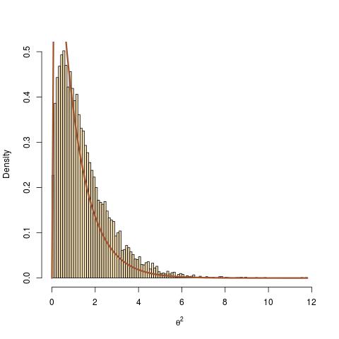
More central to the point raised by the question, I find the question utterly interesting and my first solution would have been yours, namely to use the Dirac mass transform of $(\theta,y)$ into $x$. However, it does not work as shown by the following toy example where one starts with a normal observation$$x\sim\mathcal{N}(0,\theta^{-2})$$ and an exponential prior on $\theta^2$, $$\theta^2\sim\mathcal{E}(1)$$ It is a standard derivation to show that the posterior distribution on $\theta^2$ [or conditional of $\theta^2$ given $x$ if you prefer] is a Gamma distribution$$\theta^2|x\sim\text{Ga}(3/2,1+x^2/2)$$Now, if one considers the transform $y=\theta x$, then $y|\theta\sim\mathcal{N}(0,1)$, which means that the distribution of $y$ does not depend on $\theta$, hence that $\theta$ and $y$ are independent. In summary, my toy example involves the distributions $$\theta^2\sim\mathcal{E}(1)\quad x\sim\mathcal{N}(0,\theta^{-2})\quad y=\theta x\sim\mathcal{N}(0,1)$$ which means that the posterior on $\theta$ given $y$ is the prior

The R code following your suggested implementation is

y=rnorm(1) #observation
T=1e4 #number of MCMC iterations
the=rep(1,T) #vector of theta^2's
for (t in 2:T){ #MCMC iterations
  #step 2(a)
  #true conditional of x on θ:
  x=y/sqrt(the[t-1]) 
  #step 2(b) with no R
  #true conditional of θ on x:
  the[t]=rgamma(1,shape=1.5,rate=1+.5*x^2)}

leads to a complete lack of fit. Actually, the lack of fit can be amplified by choosing a very large value for $y$.

The intuitive (and theoretically valid) explanation for this lack of fit is that the Gibbs sampler (or equivalently another MCMC sampler) should always condition on $y$, the sole observation. Therefore, when computing $x$ as a deterministic transform of $(y,\theta)$, this has no impact on the distribution of $\theta$ given $x$ and $y$: it is the same as the distribution of $\theta$ given $y$, given the Dirac on $x$.

In conclusion, the correct version of your algorithm is as follows:

1. choose initial $\Theta^{(0)}$; m=0
2. while m $\leq$ NMaxIterations do {
   (a) transform $X^{(m)} = g^{-1}(y; \Theta^{(m)})$
   (b) sample
   $R^{(m+1)} \sim p(R | \Theta^{(m)}, y)$ , and then
   $\Theta^{(m+1)} \sim p(\Theta | R^{(m+1)}, y)$
   (c) m=m+1 }
3. $\Theta^* = \text{mean}((\Theta^{(N_B)}, ..., \Theta^{(NMaxIterations)}))$, where $N_B$ is some burn-in period.

This clearly means that the completion step 2(a) is unnecessary.

Answer 2

If you transform a random variable then there's certainly a Jacobian if you're calculating the density from that of the original variable (conditional or otherwise).

Here I consider a monotonic increasing transform $t()$; the case for a decreasing one is similar but involves a small extra step.

Consider $X\sim F_X$ and the transformation $Y=t(X)$.

$F_Y(y) = P(Y\leq y) = P(t(X)\leq y) = P(X\leq t^{-1}(y)) = F_X(t^{-1}(y))$

when you differentiate back to a density, you can see where the Jacobian comes from:

$f_Y(y) = \frac{d}{dy} F_X(t^{-1}(y))=f_X(t^{-1}(y)) \cdot \frac{d}{dy}t^{-1}(y)$

... that last term is a Jacobian.

Now if $t$ is decreasing, and you follow the above argument through, you get a minus sign come in; the general univariate case for invertible transformations will then place an absolute value ( $|.|$) around the Jacobian which will work either way. (The multivariate case is quite similar)

You can see from following through the above argument that conditioning will carry through.

If the transformation is not 1 to 1, things become somewhat more complicated.