6
$\begingroup$

I am interested in using the results from this paper (Modified exact sample size for a binomial proportion with special emphasis on diagnostic rest parameter estimation by Geoffrey Fosgate) to calculate sample sizes. There is an implementation of the algorithm used to calculate the sample size in R's binomSamSize package. I have checked the code used to calculate this and it seems to follow the paper exactly, but the results shown in the paper's results section do not seem to be reproducible. The sample sizes turn out to be too small.

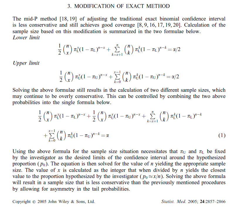
The paper requires a subscription to be viewed in it's entirety, but here is a snippet to show how the sample size is calculated:

enter image description here

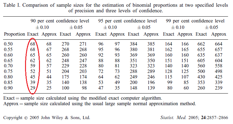
Here are the results I want to reproduce: enter image description here
Here is the code I am using (lifted from the binomSamSize package):

ciss.midp <- function(p0, d, alpha, nMax = 1e+06){
  pi.L <- p0 - d
  pi.U <- p0 + d
  if (pi.L < 0) 
    stop("p0 - d is below zero!")
  if (pi.U > 1) 
    stop("p0 + d is above one!")
  n <- floor(max(1/p0, 1/(1 - p0)))
  done <- FALSE
  while (!done & (n < nMax)) {
    n <- n + 1
    x <- round(p0 * n)
    lhs2 <- 1/2 * dbinom(x, size = n, prob = pi.L) + 1/2 * 
      dbinom(x, size = n, prob = pi.U) + 
      pbinom(x, size = n, prob = pi.L, lower.tail = FALSE) + 
      pbinom(x - 1, size = n, prob = pi.U)
    if (!is.na(lhs2)) {
      done <- (lhs2 < alpha)
    }
  }
  return(n)
}

What I end up getting to produce the circled column is this:

> sapply(seq(0.5, 0.9, 0.05), function(i) ciss.midp(p0=i, d=0.1, alpha=0.1))
[1] 68 67 65 61 57 50 42 34 23

PS: If there is anything else I can provide to make this easier to answer, please let me know in the comments.

$\endgroup$
3
  • 2
    $\begingroup$ Posting relevant portions of papers is considered fair use almost everywhere (although I am told that laws vary from country to country). It would be unlikely to raise objections here. Posting the entirety of a paper would be frowned on. $\endgroup$
    – whuber
    Commented Dec 15, 2015 at 20:53
  • $\begingroup$ @whuber Thanks for the quick response. I added the relevant snippet. $\endgroup$
    – statsNoob
    Commented Dec 15, 2015 at 21:01
  • $\begingroup$ Nothings seems to be off. You best bet is to contact the authors. $\endgroup$ Commented Dec 15, 2015 at 23:33

1 Answer 1

3
$\begingroup$

Maybe the author's implementation - despite the description - starts with a large n and works back and stops at the first time we are above alpha, thus returning the last n where the sum was below alpha? At least an implementation of such an algo would be consistent with the results of the paper (test code below).

There appear to be more than one n, where a switch from the sum being above alpha for n and being below alpha for n+1... However, I do think it's better to go from small n and up.

##Go the other way...not my 1st choice though...
ciss.midp2 <- function (p0, d, alpha, nMax = 1e+05) {
    pi.L <- p0 - d
    pi.U <- p0 + d
    if (pi.L < 0)
        stop("p0 - d is below zero!")
    if (pi.U > 1)
        stop("p0 + d is above one!")
    n <- nMax
    done <- FALSE
    while (!done & (n > 0)) {
        n <- n - 1
        x <- round(p0 * n)
        lhs2 <- 1/2 * dbinom(x, size = n, prob = pi.L) +
          pbinom(x, size = n, prob = pi.L, lower.tail = FALSE) +
          (1 - pbinom(x-1, size = n, prob = pi.U, lower.tail=FALSE)) +
          1/2*dbinom(x, size = n, prob = pi.U)

        if (!is.na(lhs2)) {
            done <- (lhs2 > alpha)
        }
    }
    return(n+1)
}

library("binomSamSize")
p.grid <- seq(0.5, 0.9, 0.05)
sapply(p.grid, function(i) ciss.midp(p0=i, d=0.1, alpha=0.1))
[1] 68 67 65 61 57 50 42 34 23
sapply(p.grid, function(i) ciss.midp2(p0=i, d=0.1, alpha=0.1)
[1] 68 67 65 61 57 52 45 39 29
$\endgroup$
3
  • $\begingroup$ Thanks for answering. This makes sense, but when I try to replicate another result in the same table, I don't get the same results again. To replicate the 99% confidence level at 0.05 margin of error, sapply(seq(0.5, 0.9, 0.05), function(i) ciss.midp2(i, 0.05, 0.01)) gives 662 654 635 603 560 503 434 358 268 instead of the author's result 662 655 635 605 560 500 430 353 260 $\endgroup$
    – statsNoob
    Commented Dec 17, 2015 at 12:35
  • $\begingroup$ Maybe part of the problem is the numerical precision of the different implementations (R vs. Fortran)? Still, in R I'd go for the R ciss.midp function, for example: > p0 <- 0.85 ; d <- 0.05 ; x <- round(p0*n) ; alpha <- 0.01 > (n <- ciss.midp(p0=p0, d=d, alpha=alpha)) [1] 342 > 1/2 * dbinom(x, size = n, prob = pi.L) + 1/2 * + dbinom(x, size = n, prob = pi.U) + pbinom(x, size = n, + prob = pi.L, lower.tail = FALSE) + pbinom(x - 1, + size = n, prob = pi.U) [1] 0.009965654 Maybe try to get the Fortran code from the author? $\endgroup$
    – mhoehle
    Commented Dec 19, 2015 at 15:53
  • $\begingroup$ I got the author's Fortran code. It is largely posted here: stackoverflow.com/questions/34619962/… $\endgroup$
    – statsNoob
    Commented Jan 5, 2016 at 19:45

Your Answer

By clicking “Post Your Answer”, you agree to our terms of service and acknowledge you have read our privacy policy.

Not the answer you're looking for? Browse other questions tagged or ask your own question.