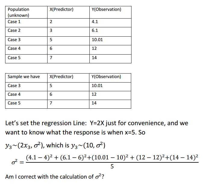
The first slide is the denifition of simple linear regression model, the second slides is an example
[![definition][1]][1]
 The second question I have is I still have difficulties in understanding Confidence interval for mean and Confidence interval and Prediction interval. For the example above, if I was correct,the standard deviation would be 0.0634 then y3 would be :y3~(10,0.0634^2), so we can say we are 95% sure y3 would be from 10-2*0.0634 to 10+2*0.0634, why we still need Confidence interval for mean and and Prediction interval?
 Why we can't just use standard deviation s from sample directly
2 Answers
You should distinguish two concepts; (1) you have a ''model'', i.e. assumptions that you make about what the ''real world'' is like and (2) you estimate the model from sample data.
Let us use an example: I think that the weight ($W$) of a person depends on his length ($L$). This seems like a reasonable assumption, however it is not precise enought to make it a ''model''. Therefore I will assume that $W = \beta_0 + \beta_1 L$. This looks like a ''good'' model but there is something missing: if this would be the description of the ''real world'' then it would mean that all persons with length $L=1.8$ meter would have exactly the same weight namely $\beta_0+\beta_1 \times 1.8$. I am sure that you will agree that not all the people with $L=1.8$ have all the same weight, so we have to ''complete'' this model. The additional assumption is that the people with $L=1.8$ must not all have the same weight, it may be different but we assume that the weights of all people with length $L=1.8$ are normally distributed with a mean $\beta_0 + \beta_1 \times 1.8$ and an (unknown) standard deviation $\sigma$ and we assume that this $\sigma$ is the same for all persons.
So our model becomes $ W = \beta_0 + \beta_1 L + \epsilon$, where $\epsilon \sim N(0;\sigma)$ or, equivalently $W \sim N(\beta_0 + \beta_1 L;\sigma)$.
The values for $\beta_0, \beta_1, \sigma$ are unknown values. To have ''an idea'' about these values, we will have to estimate their values from a sample (you need a sample because you can not measure and weight all the people in the world). So let us take a sample of e.g. $n=50$ persons and measure their weight ($W_i, i=1,2,\dots,n$) and length weight ($L_i, i=1,2,\dots,n$). With ordinary least squares regression (OLS) one can now compute ''estimates'' for these unknown values, i.e. $\hat{\beta_0}, \hat{\beta_1}, \hat{\sigma}$. The ''hat'' shows that these are estimates, so they are not the ''true'' values, these ''true values'' are unknown.
If I would take another sample of 50 (other) persons, then I will obviously find other values for these estimates ... So they are not known exactly, they behave ''random''.
If I now want to ''predict'' the weight of a person of 1.75m, then my guess would be $\hat{W} = \hat{\beta_0} + \hat{\beta_1} \times 1.75$.
But the $\hat{\beta_0}$ and $\hat{\beta_1}$, are obtained from a sample, and if I draw another sample then I will find other values for these $\hat{\beta_i}$ and therefore also other values for my prediction $\hat{W}$. So this $\hat{W}$ is also behaving ''random''.
So the prediction $\hat{W}$ will change everytime you draw another sample of $n=50$ persons. Therefore you should compute a confidence interval.
The theory on linear regression learns that the distribution of $\hat{W}$ and this finding can be used to construct confidence intervals.
If you want an explanation on how to interpret a confidence interval see section 3 of Why is there a need for a 'sampling distribution' to find confidence intervals?.
In the example that you are giving you assume the model $Y=\beta X + \epsilon$ and you also assume that you know that $\beta = 2$. The latter is usually not known, you will have to estimate this value from your sample data and find a value $\hat{\beta}$ that will change when you compute it from another sample.
EDIT: after the additional question in your comment
Assume the you would know the $\beta_0$ and $\beta_1$ exactly, then your model tells you that $W \sim N(\beta_0 + \beta_1 L, \sigma)$. So if you know $\beta_0$, $\beta_1$ and $\sigma$ exactly then you could do as in your comment and make a confidence interval of $[\beta_0 + \beta_1 1.75 - 1.96\sigma;\beta_0 + \beta_1 1.75 + 1.96\sigma]$ .
But you do not know $\beta_0$, nor $\beta_1$ (nor $\sigma$), and you have to use estimates $\hat{\beta}_0, \hat{\beta}_1$ and if you use these values in stead of the true but unkown $\beta_0, \beta_1$ then you ''introduce'' an additional error and thus additional ''uncertainty'' which will imply a wider confidence interval that is given by the complicated formula you refer to.
So if you would know the ''true'' $\beta_i$ you can compute the confidence interval as you describe. But you do not know these values, you estimate $\hat{\beta}_i$ from a sample and you use these estimates as if they are the ''true'' values, so you ''introduce'' an error.
If, in addition to replacing the $\beta_i$ by $\hat{\beta}_i$ you also estimate the $\hat{\sigma}$ then the 1.96 should be replaced by 2 because you ''introduce'' another error when you replace $\sigma$ by the (random) $\hat{\sigma}$. For another sample, you will find another value of $\hat{\sigma}$.
So, if you would know the $\beta_i$ and $\sigma$ exactly, then the formula for the 0.95 confidence interval would be $\hat{y} \pm 1.96 \sigma$, if you replace $\sigma$ by $\hat{\sigma}$ then it should be $\hat{y} \pm 2 \hat{\sigma}$ and if I use the $\hat{\beta}_i$ to compute $\hat{y}$ then you also get the square root factor.
Maybe this will make it a bit clearer (but it is not exact, it more intuitive): assume that your real world (which we never know) would be $W \sim N(\beta_1L, \sigma)$. and thet $\beta_1=2$. I invite you to make a graph $y=2x$ and draw a confidence interval $\pm 1.96\sigma$ (take e.g. $\sigma=1$)., these are two parallel lines.
In reality you don't know that $\beta_1=2$ and you will estimate it from a sample, maybe you will find $\hat{\beta}_1=1.99$, now draw the line $y=1.99x$ and the confidence bands $\pm 1.96\sigma$.
If you take another sample, you will find another $\hat{\beta}_1$, e.g. $\hat{\beta}_1=2.01$, draw the lines for these values. Then the combination of all these ''confidence bands'' gives you ... a wider and curved confidence band (if you do this for $\hat{\beta}_1=1.95, 1.96, ... 2.05$).
-
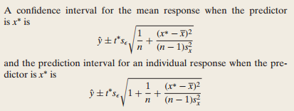
$\begingroup$ many thanks for your detailed answer. It really helped a lot. One last thing I don't get is, let's say we estimate the sample deviation s, then we can from the model of W^=β0^+β1^×1.75 we have one response value w^ when predictor is 1.75, then we can say 95% the true weight value will be from w^-2s to w^-2s (I know the t value should not be 2,as the df is n-2, but let's have it for convenience). why we still have some complicated formula like s\sqrt{\frac{1}{n}+\frac{{(x*-x)}^2}{(n-1)S_{x}^{2}}}, why don't we just simply use s? $\endgroup$– whoisitCommented Dec 22, 2015 at 1:17
-
$\begingroup$ sorry I don't know how to type the math symbol, you know we have a formula instead of use s directly, I will add the picture in my question $\endgroup$– whoisitCommented Dec 22, 2015 at 1:23
-
$\begingroup$ @whoisit: I have edited the answer $\endgroup$– user83346Commented Dec 22, 2015 at 10:01
-
$\begingroup$ Thank you so so much for your answer, it really help me so much $\endgroup$– whoisitCommented Dec 22, 2015 at 11:13
-
$\begingroup$ @whoisit: you're welcome, glad I could help you and if you like the answer, don't forget to vote for it or if you realy like it, make it your best answer $\endgroup$– user83346Commented Dec 22, 2015 at 11:34
You have sample data so the variance equation is actually divided by (N-2). There's a short article here that talks about this calculation.
-
$\begingroup$ do you mean it should be divided by 3 not 5?. But that is for population, not sample, isn't it? $\endgroup$– whoisitCommented Dec 20, 2015 at 7:20
-
$\begingroup$ @whoisit you should divide by 5 if it's the population or 3 if it's a sample. $\endgroup$ Commented Dec 20, 2015 at 7:31
-
$\begingroup$ what I have in my example is for the population, so I think it should be divided by 5. Could you please have a look at my second question about two intervals? Thank you $\endgroup$– whoisitCommented Dec 20, 2015 at 7:46
-
$\begingroup$ @whoisit: you say that $Y=2X$, now it all depends: usually you state that $Y=\beta X$ and you do not know the ''true'' $\beta$ therefore you estimate it from your data. This estimated value differes from the true value therefore it is denoted $\hat{\beta}$. For every value $\beta$ that you estimate from the data, you have to subtract 1 from $N$. So if you are sure that $\beta=2$ then it is $N$ because you know it is 2, so you did not estimate , if $\hat{\beta}=2$ is estimated from the data then you have to subtract 1. In the link there are two $\beta$'s that are estimated from the data. $\endgroup$– user83346Commented Dec 20, 2015 at 15:34
-
$\begingroup$ @fcop thanks for your answer. Could you please have a look at my second question about two intervals? Thank you $\endgroup$– whoisitCommented Dec 21, 2015 at 1:40
