Distribution of values in a time series (tidal data)

Question

I was trying to help my colleague with fitting a distribution curve to some empiric data (these are sea water level observations at different time points). However, I haven't succeeded since it's my first experience in approximating an empiric distribution with a theoretical one.

The mean value of $Y$ is 0.32688.

$\sigma^2_Y$ is 0.076191.

Here's a histogram:

And an empirical cdf:

There are 1024 samples in the data.

Obviously the distribution is asymmetric. It doesn't look like $\chi^2$ since $\hat{\mu}_Y >> 2\hat{\sigma}_Y^2$

I tried approximating it with beta distribution (picked various $\alpha, \beta$ parameters) together with normalizing Y by some real number in $[0.5; 3]$. It didn't help, Pearson chi-squared statistic was always, you know, like 300, 700 or even more.

I tried squaring Y and the histogram of $Y^2$ looks like this:

I tried approximating this with exponential distribution (and normalizing Y with a real number) - but P-value was always like zero all the time.

The data itself can be found here: https://docs.google.com/spreadsheet/ccc?key=0AqeuZRXRoMfRdF9UQzFEZVdOTmh0ZzNSaFRhRndHWmc

Does anyone have any ideas on what distribution this data could have?

Answer 1

Tides not only have periods of little bit above 24 hours (due to earth rotation). If you do a Fourier decomposition of tidal readings you'll see that there are harmonics with a a far longer period that are not multiple of the main one. Also there is a Syzygy involving Earth, Moon and Sun every 28 days or so which affects tides (of course is coastal geography dependent but still). This is a pic from wikipedia more illustrative that my verbal skills.

Quick edit: actually, Wikipedia's page section on tides' analysis is far more illustrative than my comment.....

Answer 2

Distribution calculated from a periodic function

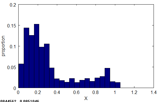
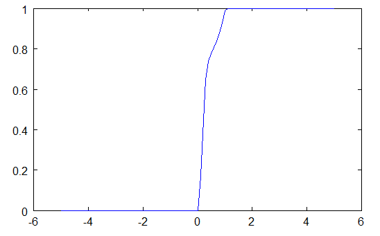
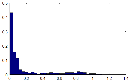
Your water height data is some recurring pattern that can be modeled in various ways. From these models for the data you could obtain a distribution which is slightly more intuitive/direct/correct in comparison to directly trying to guess and fit a distribution to the histogram.

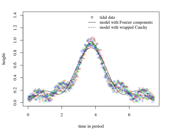
The recurring pattern is best viewed when you overlay all the cycles, which can be done by plotting against the time variable modulo the cycle period. See in the image below your data with two fitted models that are explained later.

Your data seems to be 7.5 points per day. But the tidal period is slightly less by almost a fraction 1/365 (I got to this by splitting the data in thirds, that is the origin for the colors in the image, and aligning them by changing the parameter manually). ^{(which is actually strange since one would expect the period to be longer by the lunar cycle and an extra 1/29).}

Time of sampling as a random variable

The result of the mismatch between the cycle period and the sampling frequency is that you may be taking time measurements every day at the same point, but this is a different point in the cycle each time.

You could consider the time to take a sample as a random variable $T$ that is uniform distributed between 0 and the period of the cycle $\frac{1}{\nu}$.

$$T \sim \text{Unif}(0,\frac{1}{\nu})$$

Height as a transformed variable with added noise

The tidal wave height $Y$ can be seen as variable that results from a transformation of the time variable $T$ and with some added noise:

$$y_i = g(t_i) + \epsilon_i$$

Once you know the function $g$ and the distribution of the noise $\epsilon$ then you can use the standard transformation rules to obtain the distribution of the measured heights variable $Y$.

• Transformation with $z = g(t)$ and inverse $t = g^{-1}(z)$ you can describe the probability distribution function of $Z$ in terms of the probability distribution function of T: $$f_Z(z) = f_T(g^{-1}(z)) \left|\frac{\text{d}g^{-1}(z)}{\text{d}z}\right| $$ ^{Intuition: the values at a steep slope of the curve are relatively less likely because they are more spread out}

• Summation $Y=Z+\epsilon$ is a sum of two variables. Then the resulting pdf can be described as a convolution.

---

Example 1: Fourier cosine series

Because of the symmetry in the pattern of the wave in the image above I decided to model the function as a sum of cosine functions:

$$y(t) = \sum_{k=0}^{k=K} a_k cos(2k\pi \nu t) $$

where I used the first five components

a_0   =   0.32687
a_1   =  -0.32842
a_2   =   0.16507
a_3   =  -0.08664
a_4   =  -0.02772

The inverse transformation formula $g^{-1}(t)$ is a bit awkward here. It is multivalued and also difficult to obtain analytically (if at all possible). But we can express the distribution function of $y$ in a different way by expressing it as a mixture of Gaussian distribution functions $f_\epsilon(y,g(t),\sigma_\epsilon^2) = \frac{1}{\sqrt{2\pi\sigma_\epsilon^2}} exp(\frac{(y-g(t))^2}{2\sigma_\epsilon^2}) $ around the means $z=g(t)$ and integrate over all possible values $t$:

$$f_Y(y) = \nu \int_0^{\frac{1}{\nu}} f_\epsilon(y,g(t),\sigma_\epsilon^2) dt$$

Example 2: Wrapped Cauchy distribution

The coefficients in the example above seemed to behave a bit like $a_k \propto \left( \frac{-1}{2} \right)^k$. This relates to the wrapped Cauchy distribution with $\gamma=\ln(2)$

$$f_{WC}(\theta,\mu,\gamma) = \frac{1}{2 \pi} \frac{\sinh \gamma}{\cosh \gamma - \cos(\theta-\mu)} $$

So I tried fitting a scaled version of this

$$y(t) = a + b \frac{0.75}{1.25 - \cos(\nu t-0.5)} $$

which worked reasonable as you can see above in the image.

The advantage of this function is that it has an inverse and this inverse is monotonic (if you just use one half) so we can do the transformation and then the convolution to obtain the distribution of $Y$:

$$f_Y(y) = \int_{\frac{1}{3}}^{3} f_\epsilon(y-z,0,\sigma_\epsilon^2) 2\nu \left|\frac{\text{d}g^{-1}(z)}{\text{d}z}\right| dz$$

^{such expression may be easier to solve analytically than the one for case 1, although here (see the code below) I still solve it computationally.}

Display of example 1 and 2

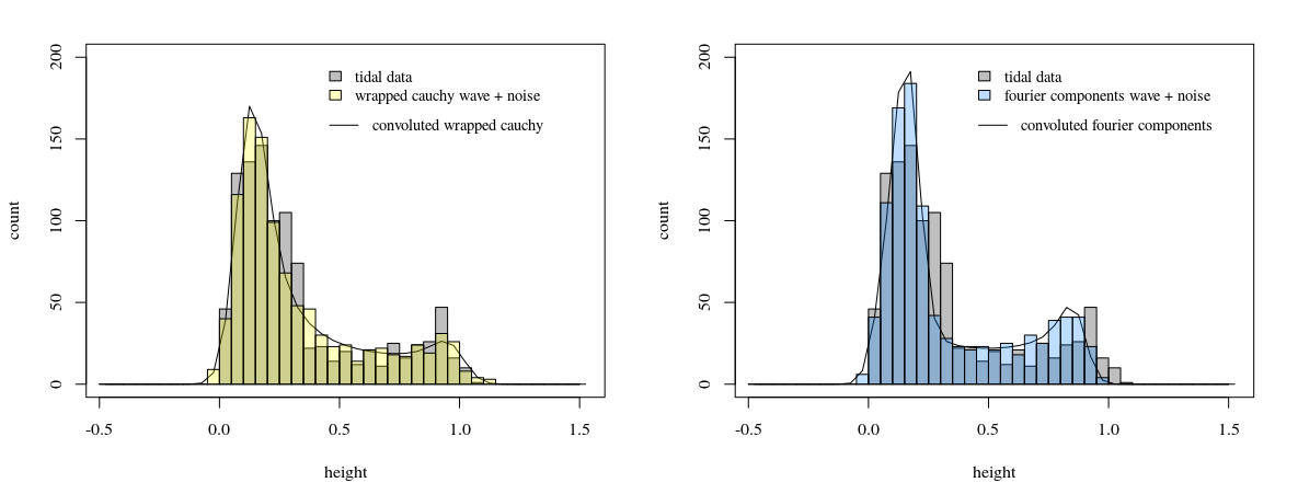
The fitted curves are shown in the image at the start. Below you see how the results are for the histogram of the data compared with (1) a modeled histogram from the fitted height function (as a sanity check for all the computations) and (2) a computed probability distribution function based on the fitted height function.

#########################################

# data
t <- 1:1024
tides <- c(0.339,1.052,0.3142,0.2563,0.2336,0.1746,0.06897,0.2611,0.7063,0.8456,0.1924,0.07416,0.1487,0.1793,0.2219,0.4221,0.937,0.3834,0.1785,0.07275,0.05573,0.1157,0.2605,0.7804,0.7169,0.2529,0.1096,0.08469,0.05687,0.19,0.4317,1,0.2699,0.2513,0.2114,0.1195,0.05203,0.2712,0.9199,0.638,0.3113,0.07248,0.04128,0.1519,0.2828,0.4129,1.022,0.2688,0.1594,0.1813,0.1824,0.1153,0.2311,0.9107,0.6396,0.1866,0.02282,0.07995,0.1048,0.2394,0.5414,0.8714,0.3164,0.1479,0.06487,0.08711,0.1501,0.3139,0.8634,0.5759,0.301,0.1704,0.08626,0.04383,0.2539,0.6663,0.8669,0.2281,0.1759,0.2206,0.1897,0.1043,0.2645,1.006,0.5225,0.321,0.2014,0.06469,0.09601,0.3132,0.5417,0.9437,0.1953,0.1866,0.1901,0.1747,0.1497,0.3368,0.9001,0.5191,0.22,0.05603,0.08189,0.1347,0.2426,0.6316,0.8285,0.2738,0.1463,0.1055,0.1047,0.1641,0.294,0.9845,0.427,0.3118,0.1797,0.03837,0.06875,0.2871,0.7374,0.8411,0.2932,0.03483,0.1374,0.1641,0.1998,0.2866,1.008,0.4357,0.2623,0.1878,0.1148,0.02958,0.2982,0.7525,0.7975,0.1788,0.06431,0.06452,0.1101,0.2098,0.399,0.9139,0.4045,0.1834,0.09027,0.117,0.1164,0.2375,0.7693,0.7474,0.3098,0.1236,0.05057,0.1171,0.2606,0.4785,0.9512,0.2663,0.2601,0.2048,0.09881,0.03758,0.3246,0.8457,0.7473,0.3376,0.09456,0.05258,0.1867,0.3124,0.3677,0.9616,0.3463,0.2546,0.1803,0.1078,0.1125,0.3358,0.8178,0.6826,0.2409,0.108,0.09618,0.08841,0.1863,0.4956,0.9156,0.3451,0.1804,0.1166,0.1083,0.1234,0.1844,0.8843,0.6243,0.3151,0.08255,0.06786,0.1626,0.2719,0.5413,0.9864,0.2677,0.138,0.1952,0.1598,0.1064,0.2573,0.8756,0.6467,0.2989,0.1184,0.03106,0.1117,0.317,0.5398,0.9133,0.2167,0.105,0.07625,0.1038,0.151,0.2725,0.8668,0.5402,0.2234,0.09513,0.08771,0.06582,0.2067,0.6394,0.8712,0.3148,0.13,0.1175,0.1545,0.21,0.2964,0.9524,0.4283,0.3193,0.1297,0.02149,0.1527,0.3474,0.6428,0.9463,0.2976,0.04256,0.1427,0.2084,0.2567,0.2717,0.9287,0.5533,0.2486,0.1155,0.08158,0.1406,0.3467,0.68,0.8286,0.2863,0.1394,0.07582,0.01711,0.1371,0.3693,0.9025,0.4636,0.2602,0.1342,0.09308,0.0658,0.1726,0.7493,0.809,0.2575,0.05393,0.171,0.1875,0.2296,0.3671,1.03,0.3156,0.2533,0.2095,0.1245,0.05833,0.2979,0.7089,0.841,0.2562,0.01355,0.09313,0.1759,0.2816,0.3617,0.9663,0.361,0.1503,0.05188,0.08762,0.07043,0.2288,0.7679,0.7145,0.2416,0.1001,0.07742,0.03327,0.1846,0.5002,0.9408,0.3241,0.1994,0.1792,0.148,0.1289,0.2206,0.8657,0.6255,0.3251,0.0587,0.1261,0.2083,0.3041,0.4186,1.037,0.2937,0.1651,0.1862,0.1939,0.137,0.2425,0.8272,0.7051,0.1905,0.02176,0.1164,0.1939,0.3218,0.4954,0.9064,0.3438,0.1539,0.0743,0.05751,0.1201,0.2925,0.8342,0.6424,0.3118,0.1436,0.08717,0.02174,0.1801,0.5702,0.9071,0.2121,0.1842,0.2186,0.1637,0.1366,0.2684,0.9965,0.4973,0.3283,0.1625,0.0469,0.1117,0.3084,0.5395,0.947,0.2328,0.1524,0.1656,0.1903,0.1759,0.247,0.9064,0.5207,0.1792,0.005314,0.0599,0.04464,0.2497,0.6152,0.8556,0.2547,0.1557,0.07076,0.06686,0.1734,0.3401,0.9156,0.444,0.3001,0.1697,0.1057,0.0161,0.2297,0.7152,0.7958,0.2665,0.09849,0.2,0.2258,0.1753,0.2868,1.016,0.4377,0.2534,0.2051,0.1172,0.03664,0.2825,0.6658,0.8307,0.1642,0.1066,0.1609,0.1904,0.259,0.3692,0.9445,0.4603,0.1657,0.08144,0.08947,0.1193,0.2429,0.7228,0.775,0.3239,0.1382,0.1025,0.08795,0.2041,0.391,0.9413,0.3388,0.2585,0.1839,0.08396,0.08986,0.2914,0.8682,0.7043,0.3421,0.05705,0.08206,0.1693,0.2804,0.3941,0.9714,0.3688,0.2585,0.1835,0.1153,0.08032,0.2682,0.7812,0.7123,0.1663,0.05597,0.05723,0.06999,0.2253,0.4266,0.9418,0.3075,0.1894,0.08753,0.1101,0.1258,0.2056,0.8504,0.6465,0.3265,0.1161,0.04002,0.09416,0.2544,0.535,0.9014,0.2795,0.2207,0.2172,0.183,0.05627,0.3212,0.8959,0.6651,0.3177,0.1408,0.0389,
           0.1005,0.2999,0.4975,0.9255,0.2661,0.1892,0.1396,0.1537,0.1603,0.3138,0.8838,0.5826,0.2041,0.1081,0.08694,0.09003,0.1745,0.5948,0.8872,0.3121,0.1571,0.1416,0.1443,0.1857,0.2417,0.9241,0.5298,0.2861,0.1024,0.04219,0.1403,0.3066,0.6824,0.8944,0.288,0.06598,0.1895,0.2009,0.2099,0.2735,0.9147,0.5382,0.2774,0.1204,0.03039,0.1201,0.3084,0.6331,0.8643,0.1951,0.1305,0.06724,0.1031,0.1708,0.2819,0.9453,0.4553,0.2231,0.07429,0.08636,0.07272,0.1844,0.7189,0.8026,0.2799,0.08854,0.1308,0.1864,0.2276,0.3652,0.9475,0.3914,0.28,0.2057,0.06863,0.06225,0.3571,0.7141,0.8623,0.3074,0.06423,0.07923,0.1575,0.2895,0.3257,0.9552,0.4189,0.2247,0.08396,0.09051,0.1182,0.3183,0.7603,0.7186,0.2369,0.1274,0.09098,0.0649,0.1412,0.4545,0.923,0.3744,0.2482,0.1828,0.129,0.1295,0.1693,0.842,0.6945,0.2793,0.05112,0.1381,0.1797,0.253,0.4654,1.015,0.2862,0.2099,0.2173,0.1869,0.114,0.2761,0.8169,0.7266,0.2236,0.01275,0.092,0.191,0.293,0.4488,0.9308,0.299,0.1818,0.06981,0.08649,0.1191,0.2386,0.8629,0.6281,0.2288,0.06733,0.0669,0.003544,0.1776,0.5635,0.9185,0.248,0.1772,0.1934,0.1825,0.1588,0.2431,0.9158,0.5436,0.3005,0.1145,0.07198,0.1757,0.3305,0.5012,0.9876,0.316,0.1303,0.1693,0.1938,0.1907,0.212,0.9179,0.5724,0.1933,0.02915,0.1011,0.1388,0.2896,0.6212,0.8455,0.2948,0.142,0.04251,0.04993,0.1376,0.3536,0.9036,0.5224,0.3083,0.1819,0.09134,0.02542,0.1688,0.7084,0.8219,0.2273,0.1402,0.2102,0.1664,0.1493,0.3229,1.022,0.4026,0.3077,0.2337,0.09662,0.08126,0.3191,0.6421,0.8527,0.1863,0.1201,0.1431,0.1833,0.2018,0.3279,0.9337,0.4556,0.1871,0.04757,0.09425,0.09652,0.2252,0.7195,0.7866,0.2272,0.08473,0.06814,0.05251,0.1515,0.3754,0.9413,0.3465,0.2787,0.1731,0.1086,0.03706,0.2656,0.8362,0.7246,0.2856,0.0612,0.145,0.1978,0.2594,0.3213,1.023,0.3975,0.2263,0.2088,0.144,0.04885,0.2396,0.7854,0.7338,0.1612,0.06516,0.1124,0.1508,0.2521,0.4623,0.9143,0.384,0.1544,0.02236,0.08462,0.1233,0.297,0.8169,0.6965,0.3544,0.141,0.0752,0.1015,0.2327,0.5265,0.899,0.26,0.2444,0.2066,0.125,0.03576,0.276,0.9219,0.622,0.347,0.1671,0.01027,0.1719,0.2977,0.4494,0.9386,0.2928,0.1998,0.1596,0.1108,0.1132,0.3014,0.8423,0.6317,0.207,0.03396,0.07801,0.1061,0.2302,0.5691,0.8831,0.273,0.1567,0.1055,0.05348,0.1057,0.2281,0.9027,0.5527,0.2895,0.1141,0.03285,0.0963,0.2849,0.6563,0.8747,0.2562,0.1356,0.1946,0.1687,0.1248,0.2468,0.9875,0.5658,0.2835,0.1552,0.0687,0.07856,0.309,0.6059,0.8819,0.1714,0.1303,0.1022,0.1271,0.1907,0.3613,0.916,0.4823,0.1665,0.08353,0.1072,0.1223,0.2654,0.6609,0.8289,0.3384,0.1126,0.144,0.1636,0.2389,0.3372,0.9454,0.4003,0.3021,0.1748,0.0325,0.1025,0.3046,0.7427,0.852,0.3393,0.04777,0.1026,0.2148,0.2702,0.2975,0.9362,0.4757,0.2533,0.1026,0.06041,0.1097,0.3035,0.7233,0.7938,0.2347,0.1102,0.1022,0.0963,0.1899,0.4139,0.9104,0.3723,0.2021,0.1145,0.05765,0.03492,0.187,0.7954,0.7611,0.2788,0.05129,0.1149,0.1794,0.2432,0.4415,0.9828,0.2882,0.204,0.2025,0.1205,0.01877,0.2947,0.8422,0.7623,0.3023,0.0681,0.06518,0.1645,0.3174,0.4116,0.9761,0.2924,0.1881,0.07769,0.1002,0.1484,0.2772,0.8284,0.616,0.2348,0.1134,0.08772,0.09173,0.2204,0.5293,0.932,0.345,0.1661,0.2013,0.1867,0.1599,0.2088,0.9284,0.5698,0.3196,0.09019,0.09065,0.1897,0.3027,0.541,1.011,0.2792,0.1242,0.2015,0.2123,0.1794,0.2324,0.8494,0.6735,0.2373,0.02838,0.07939,0.147,0.3001,0.5681,0.8868,0.2881,0.1688,0.09133,0.04628,0.1405,0.2936,0.8688,0.542,0.24,0.09419,0.06518,0.03157,0.1798,0.6081,0.9074,0.2291,0.1381,0.1857,0.1658,0.1621,0.2769,0.9998,0.413,0.2652,0.1578,0.04791,0.0938,0.33,0.6376,0.9284,0.2587,0.05157,0.145,0.2007,0.2446,0.2299,0.9797,0.4437,0.2026,0.05072,0.08956,0.1027,0.2402,0.7086,0.775,0.2818,0.1171,0.05067,0.07458,0.1631,0.4042,0.9336,0.4207,0.2605,0.201,0.1407,0.05957,0.1871,0.8211,0.7203,0.269,0.08088,0.1906,0.2176,0.2401
)

# shift the time and take the modulus
period <- 7.5*(1-1.2/365.25)
mt <- (t+1.8)%%(period)


#plot data with colours for three diffferent periods
layout(matrix(1))
plot(mt[1:340],tides[1:340],pch=21,col="NA",bg=rgb(1,0,0,0.2),
     xlim=c(0,period),ylim=c(0,1.4),
     xlab="time in period",ylab="height")
points(mt[341:680],tides[341:680],pch=21,col="NA",bg=rgb(0,1,0,0.2))
points(mt[681:1020],tides[681:1020],pch=21,col="NA",bg=rgb(0,0,1,0.2))

# time variable for plotting curves
ts <- seq(0,7.5,0.1)

# fourier components
coefs <- c(0.32687,
          -0.32842,
           0.16507,
          -0.08664,
          -0.02772)
four <- rep(0,length(ts))
for (i in 1:length(coefs)) {
  four <- four+coefs[i]*cos((i-1)*2*pi*ts/period)
}
lines(ts,four)

# wrapped cauchy (when the coefficients are like (-0.5)^n)
gam <- log(2)
wc <- sinh(gam)/(cosh(gam)-cos(pi*2*(ts/period-0.5)))
wc <- 0.75/(1.25-cos(pi*2*(ts/period-0.5)))  #using simplified notation for sinh and cosh
lines(ts,0.330259*wc-0.003385,col=1,lty=2)


legend(3.5, 1.45, c("tidal data","model with Fourier components","model with wrapped Cauchy"), 
       pch=c(21,NA,NA),lty=c(NA,1,2),box.col =NA, bg = NA, cex=0.9)



# fitting fourier components
m1 <- lm(tides ~ 1 +
           I(cos(2*pi*mt/period)) +
           I(cos(4*pi*mt/period)) + 
           I(cos(6*pi*mt/period)) +
           I(cos(8*pi*mt/period)) +
           I(cos(10*pi*mt/period))+
           I(cos(12*pi*mt/period))+
           I(cos(14*pi*mt/period))
   )

# fitting wrapped cauchy
m2 <- lm(tides ~ 1 + I(sinh(gam)/(cosh(gam)-cos(-pi+2*pi*mt/period))))



#pars
de <-   sqrt(var(m2$residuals)*1022/1021)   # variance of noise
gam <-  log(2)                              # wrapped cauchy parameter
cl <-   0.330258742                         # length scaling
ct <-  -0.003385188                         # height offset

# modelling data using wrapped cauchy + noise 
wc <- sinh(gam)/(cosh(gam)-cos(pi*2*(mt/period)))
modsig <- ct+cl*wc+rnorm(1024,0,de)

de2 <-   sqrt(var(m1$residuals)*1018/1017)   # variance of noise

# modelling data fourier components + noise 
coefs <- c(0.32687,
           -0.32842,
           0.16507,
           -0.08664,
           -0.02772)
four <- rep(0,length(mt))
for (i in 1:length(coefs)) {
  four <- four+coefs[i]*cos((i-1)*2*pi*mt/period)
}
modsig2 <- four+rnorm(1024,0,de2)

# compute histograms
h1 <- hist(tides,breaks=seq(-0.5,1.5,0.05))      # tidal data
h2 <- hist(modsig,breaks=seq(-0.5,1.5,0.05))     # wrapped cauchy
h3 <- hist(modsig2,breaks=seq(-0.5,1.5,0.05))     # fourier components

# convoluting differentiated inverse wrapped cauchy with normal
f.Y <- function(z,mu,de) dnorm(z,mu,de)        
f.X <- function(h)   0.75/(h^2*sqrt(1-(1.25-0.75/h)^2))*period/(2*pi)
f.X <- Vectorize(f.X)
f.Z <- function(z,ct,cl,de) integrate(function(x,z) f.Y(z,ct+x*cl,de)*(f.X(x)/(0.5*period)), 
                                         lower=1/3+10^-10,upper=3-10^-10,z,stop.on.error=0)$value
f.Z <- Vectorize(f.Z)

# compound normal with wrapped cauchy (this does the same as above)
f.Y <- function(z,mu,de) dnorm(z,mu,de)        
f.X <- function(t)   0.75/(1.25-cos(pi*2*(t/period))) 
f.X <- Vectorize(f.X)
f.Z <- function(z,ct,cl,de) integrate(function(x,z) f.E(z,ct+cl*f.X(x),de)/period, 
                                      lower=0,upper=period,z,stop.on.error=0)$value
f.Z <- Vectorize(f.Z)

# coompound normal with fourier components as mean
f.E <- function(z,mu,de) dnorm(z,mu,de)
f.H <- function(t) {
  four <- 0
  for (i in 1:length(coefs)) {
    four <- four+coefs[i]*cos((i-1)*2*pi*t/period)
  }
  four
}
f.Z2 <- function(z,de) integrate(function(x,z) f.E(z,f.H(x),de)/period, 
                                      lower=0,upper=period,z,stop.on.error=0)$value
f.Z2 <- Vectorize(f.Z2)


# plotting
layout(matrix(1:2,1))
x <- seq(-0.5,1.5,0.05)

plot(x+0.025,f.Z(x+0.025,ct,cl,de)*1024*0.05,type="l",
     ylim=c(0,200),
     xlab = "height", ylab = "count")
plot( h1, col=rgb(0,0,0,1/4), add=T) 
plot( h2, col=rgb(1,1,0,1/4), add=T) 
legend(0.4, 200, c("tidal data","wrapped cauchy wave + noise"), 
       fill=c(rgb(0,0,0,1/4),rgb(1,1,0,1/4)),box.col =NA, bg = NA, cex=0.9)
legend(0.4, 170, c("convoluted wrapped cauchy"), 
       lty=c(1),box.col = NA,bg = NA, cex = 0.9)

plot(x+0.025,f.Z2(x+0.025,de2)*0.05*1024,type="l",
     ylim=c(0,200),
     xlab = "height", ylab = "count")
plot( h1, col=rgb(0,0,0,1/4), add=T) 
plot( h3, col=rgb(0,0.5,1,1/4), add=T) 
legend(0.4, 200, c("tidal data","fourier components wave + noise"), 
       fill=c(rgb(0,0,0,1/4),rgb(0,0.5,1,1/4)),box.col =NA, bg = NA, cex=0.9)
legend(0.4, 170, c("convoluted fourier components"), 
       lty=c(1),box.col = NA,bg = NA, cex=0.9)


#########################################