8
$\begingroup$

Let $\left\{X_t\right\}$ be a stochastic process formed by concatenating iid draws from an AR(1) process, where each draw is a vector of length 10. In other words, $\left\{X_1, X_2, \ldots, X_{10}\right\}$ are realizations of an AR(1) process; $\left\{X_{11}, X_{12}, \ldots, X_{20}\right\}$ are drawn from the same process, but are independent from the first 10 observations; et cetera.

What will the ACF of $X$ -- call it $\rho\left(l\right)$ -- look like? I was expecting $\rho\left(l\right)$ to be zero for lags of length $l \geq 10$ since, by assumption, each block of 10 observations is independent from all other blocks.

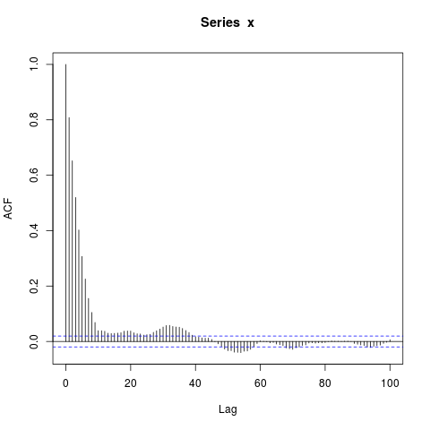
However, when I simulate data, I get this:

simulate_ar1 <- function(n, burn_in=NA) {
    return(as.vector(arima.sim(list(ar=0.9), n, n.start=burn_in)))
}

simulate_sequence_of_independent_ar1 <- function(k, n, burn_in=NA) {
    return(c(replicate(k, simulate_ar1(n, burn_in), simplify=FALSE), recursive=TRUE))
}

set.seed(987)
x <- simulate_sequence_of_independent_ar1(1000, 10)
png("concatenated_ar1.png")
acf(x, lag.max=100)  # Significant autocorrelations beyond lag 10 -- why?
dev.off()

sample autocorrelation function for x

Why are there autocorrelations so far from zero after lag 10?

My initial guess was that the burn-in in arima.sim was too short, but I get a similar pattern when I explicitly set e.g. burn_in=500.

What am I missing?


Edit: Maybe the focus on concatenating AR(1)s is a distraction -- an even simpler example is this:

set.seed(9123)
n_obs <- 10000
x <- arima.sim(model=list(ar=0.9), n_obs, n.start=500)
png("ar1.png")
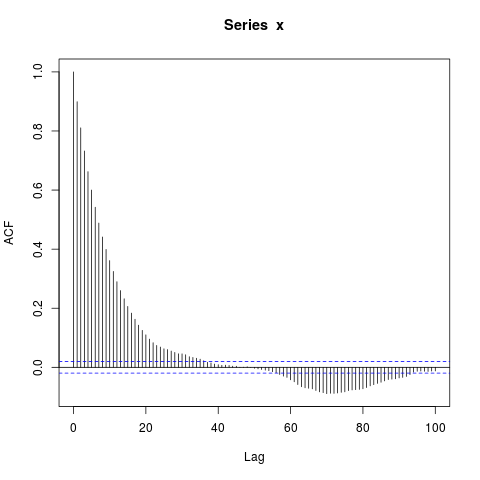
acf(x, lag.max=100)
dev.off()

acf of plain vanilla ar1

I'm surprised by the big blocks of significantly nonzero autocorrelations at such long lags (where the true ACF $\rho(l) = 0.9^l$ is essentially zero). Should I be?


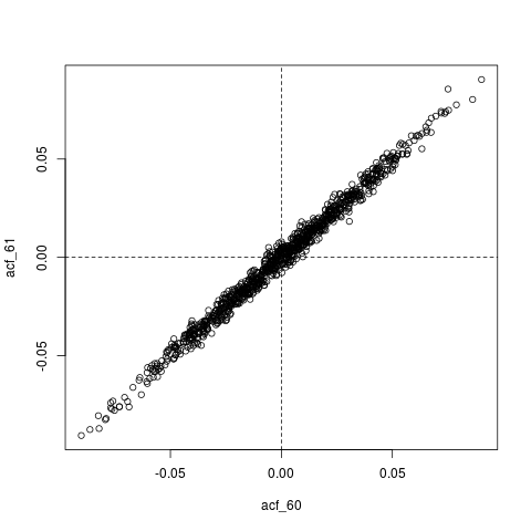
Another Edit: maybe all that's going on here is that $\hat{\rho}$, the estimated ACF, is itself extremely autocorrelated. For example, here's the joint distribution of $\left(\hat{\rho}(60), \hat{\rho}(61)\right)$, whose true values are essentially zero ($0.9^{60} \approx 0$):

## Look at joint sampling distribution of (acf(60), acf(61)) estimated from AR(1)
get_estimated_acf <- function(lags, n_obs=10000) {
    stopifnot(all(lags >= 1) && all(lags <= 100))
    x <- arima.sim(model=list(ar=0.9), n_obs, n.start=500)
    return(acf(x, lag.max=100, plot=FALSE)$acf[lags + 1])
}
lags <- c(60, 61)
acf_replications <- t(replicate(1000, get_estimated_acf(lags)))
colnames(acf_replications) <- sprintf("acf_%s", lags)
colMeans(acf_replications)  # Essentially zero
plot(acf_replications)
abline(h=0, v=0, lty=2)

sampling distribution of estimated acf

$\endgroup$
1
  • 1
    $\begingroup$ I hope my answer will still be of use to you, more than 1.5 years later. At least it helped me improve my R skills. $\endgroup$
    – Candamir
    Commented Nov 16, 2017 at 17:26

1 Answer 1

3
$\begingroup$

Executive summary: It seems that you are mistaking noise for true autocorrelation due to a small sample size.

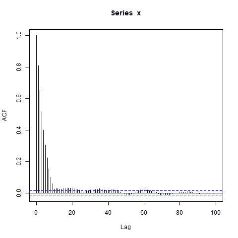
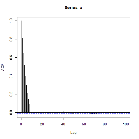
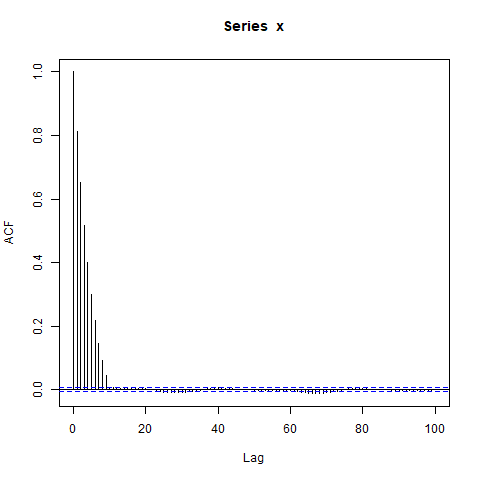
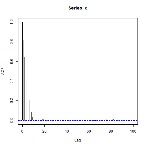
You can simply confirm this by increasing the k parameter in your code. See these examples below (I have used your same set.seed(987) throughout to maintain replicability):

k=1000 (your original code)

1000 simulations

k=2000

2000 simulations

k=5000

5000 simulations

k=10000

10000 simulations

k=50000

50000 simulations

This sequence of images tells us two things:

  • The autocorrelation after the first 10 observations greatly diminishes as the number of iterations increases. Indeed, with a sufficiently large number of iterations the $\hat\rho(l)$ for any $l>10$ will converge to zero. This is the basis for my statement at the beginning - that the autocorrelation that you observed was simply noise.
  • Notwithstanding the aforementioned observation that $\hat\rho(l)$ converges to zero for any $l>10$ as the number of simulation increases, $\hat\rho(l)$ for any $l \le 10$ actually remains constant at $\hat\rho(l)=\rho(l)=0.9^l$, just as the construction of your model would suggest.

Note that I refer to the observed autocorrelation as $\hat\rho(l)$ and to the true autocorrelation as $\rho(l)$.

$\endgroup$
5
  • 1
    $\begingroup$ The sample ACF is itself autocorrelated, so it isn't white noise. Other than that, I agree, it's just a noise / sample size issue. $\endgroup$
    – Adrian
    Commented Nov 16, 2017 at 22:44
  • $\begingroup$ @Adrian You are correct. I amended my answer accordingly. $\endgroup$
    – Candamir
    Commented Nov 16, 2017 at 22:48
  • $\begingroup$ It also becomes less and less likely to "stray" outside a confidence band -- are you sure that's true? $\endgroup$
    – Adrian
    Commented Nov 17, 2017 at 2:32
  • 1
    $\begingroup$ Thanks for poking holes into the weak parts of my answer. I have to admit that statement was only based on visual inspection. I did some further research and found out that the confidence band is calculated as qnorm((1 + ci)/2)/sqrt(x$n.used), i.e. $cdf(1-\alpha/2)/\sqrt{n}$ (see here). However, I have not been able to nail down the convergence rate for the observed autocorrelation. I asked this new question to settle the matter but have removed this point from this answer in the meantime. $\endgroup$
    – Candamir
    Commented Nov 18, 2017 at 15:56
  • 1
    $\begingroup$ @Adrian My question regarding the convergence rate of the observed autocorrelation has been answered. It turns out that its convergence rate is the same as the one of the confidence band: $1/{\sqrt{n}}$. My original claim that the observed autocorrelation becomes less and less likely to "stray" outside the confidence band is thus incorrect. That being said, the fact that $\hat\rho(l)$ converges to zero for any $l>10$ as the number of simulations increases still resolves your question, even if I was wrong about the relative rate of convergence. $\endgroup$
    – Candamir
    Commented Nov 20, 2017 at 20:45

Your Answer

By clicking “Post Your Answer”, you agree to our terms of service and acknowledge you have read our privacy policy.

Not the answer you're looking for? Browse other questions tagged or ask your own question.