14
$\begingroup$

When modeling time series one has the possibility to (1) model the correlational structure of the error terms as e.g. an AR(1) process (2) include the lagged dependent variable as an explanatory variable (on the right hand side)

I understand that their are sometimes substantial reasons to go for (2).

However, what are the methodological reasons to do either (1) or (2) or even both?

$\endgroup$

3 Answers 3

8
$\begingroup$

There are many approaches to modeling integrated or nearly-integrated time series data. Many of the models make more specific assumptions than more general models forms, and so might be considered as special cases. de Boef and Keele (2008) do a nice job of spelling out various models and pointing out where they relate to one another. The single equation generalized error correction model (GECM; Banerjee, 1993) is a nice one because it is (a) agnostic with respect to the stationarity/non-stationarity of the independent variables, (b) can accommodate multiple dependent variables, random effects, multiple lags, etc, and (c) has more stable estimation properties than two-stage error correction models (de Boef, 2001).

Of course the specifics of any given modeling choice will be particular to the researchers' needs, so your mileage may vary.

Simple example of GECM:

$$\Delta{y_{ti}} = \beta_{0} + \beta_{\text{c}}\left(y_{t-1}-x_{t-1}\right) + \beta_{\Delta{x}}\Delta{x_{t}} + \beta_{x}x_{t-1} + \varepsilon$$

Where:
$\Delta$ is the change operator;
instantaneous short run effects of $x$ on $\Delta{y}$ are given by $\beta_{\Delta{x}}$;
lagged short run effects of $x$ on $\Delta{y}$ are given by $\beta_{x} - \beta_{\text{c}} - \beta_{\Delta{x}}$; and
long run equilibrium effects of $x$ on $\Delta{y}$ are given by $\left(\beta_{\text{c}} - \beta_{x}\right)/\beta_{\text{c}}$.


References

Banerjee, A., Dolado, J. J., Galbraith, J. W., and Hendry, D. F. (1993). Co-integration, error correction, and the econometric analysis of non-stationary data. Oxford University Press, USA.

De Boef, S. (2001). Modeling equilibrium relationships: Error correction models with strongly autoregressive data. Political Analysis, 9(1):78–94.

De Boef, S. and Keele, L. (2008). Taking time seriously. American Journal of Political Science, 52(1):184–200.

$\endgroup$
5
  • $\begingroup$ The model that you are specifying can be restated as a particular case of a transfer function just as an exponential smoothing model is a particular case of an ARIMA model. Please restate your model as a dynamic regression / transfer function. $\endgroup$
    – IrishStat
    Commented Jan 24, 2015 at 14:04
  • $\begingroup$ why not ? If you constrain/specify a transfer function to a particular form you will the ECM . $\endgroup$
    – IrishStat
    Commented Jan 25, 2015 at 18:07
  • 2
    $\begingroup$ @Irish If this answer is correct, then Alexis should not feel obliged to change the explanation or cast it into some particular form. You have frequently mentioned "transfer functions," and I think I have read all your (hundreds) of posts that refer to them, but I cannot recall reading any description of what they actually are. You might consider, then, posting an answer of your own in which you explain transfer functions and show how Alexis' model can be restated in those terms. $\endgroup$
    – whuber
    Commented Jan 25, 2015 at 19:22
  • $\begingroup$ @IrishStat You have it precisely backwards: "The model that you are specifying can be restated as a particular case of a transfer function" The model you describe as a "transfer function" is a particular case of the GECM where $\beta_{x}$ has been constrained to be zero, meaning that your model assumes that the lagged effect of $x$ enters only in the equilibrium function. $\endgroup$
    – Alexis
    Commented Nov 22, 2018 at 17:27
  • $\begingroup$ ................ $\endgroup$
    – IrishStat
    Commented Nov 22, 2018 at 17:48
5
+50
$\begingroup$

This boils down to maximum likelihood vs. methods of moments, and finite sample efficiency vs. computational expediency.

Using a 'proper' AR(1) process and estimating the parameter $\rho$ (and unknown variance $\sigma^2$) via maximum likelihood (ML) gives the most efficient (lowest variance) estimates for a given amount of data.

The regression approach amounts to the Yule-Walker estimation method, which is the method of moments. For a finite sample it isn't as efficient as ML, but for this case (i.e. an AR model) it has an asymptotic relative efficiency of 1.0 (i.e. with enough data it should give answers nearly as good as ML). Plus, as a linear method it is computationally efficient and avoids any convergence issues of ML.

I gleaned most of this from dim memories of a time series class and Peter Bartlett's lecture notes for Introduction to Time Series, lecture 12 in particular.

Note that the above wisdom relates to traditional time series models, i.e. where there are no other variables under consideration. For time series regression models, where there are various independent (i.e. explanatory) variables, see these other references:

  • Achen, C. H. (2001). Why lagged dependent variables can supress the explanatory power of other independent variables. Annual Meeting of the Polictical Methodology Section of the American Politcal Science Association, 1–42. PDF
  • Nelson, C. R., & Kang, H. (1984). Pitfalls in the Use of Time as an Explanatory Variable in Regression. Journal of Business & Economic Statistics, 2(1), 73–82. doi:10.2307/1391356
  • Keele, L., & Kelly, N. J. (2006). Dynamic models for dynamic theories: The ins and outs of lagged dependent variables. Political analysis, 14(2), 186-205. PDF

(Thanks to Jake Westfall for the last one).

The general take away seems to be "it depends".

$\endgroup$
3
$\begingroup$

A good presentation of a Transfer Function (TF) is here Transfer function in forecasting models - interpretation and alternatively here http://en.wikipedia.org/wiki/Distributed_lag. Since we both have a $Y$ and one $X$ for simplicity sake then I believe that one can form a TF with appropriate assumed lags and appropriate assumed differences of these two series that would match the assumed ECM, illustrating that the ECM is a particular constrained subset of a TF model. Perhaps some other readers (heavy econometricians) have already gone thought the proof/algebra but I will consider your positive suggestion in helping other readers.

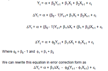
After a brief search on the web http://springschool.politics.ox.ac.uk/archive/2008/OxfordECM.pdf discussed how an ECM was a particular case of an ADL (Autoregressive Distributed Lag Model also known as a PDL). An ADL/PDL model is a particular case of a Transfer Function. This material from the above reference shows the equivalence of an ADL and ECM. Note that Transfer Functions are more general than ADL models as they allow explicit decay structure.

enter image description here

My point is that the powerful model identification features available with Transfer Functions should be used rather than assuming a model because it fits the desire to have simple explanations such as Short Run/Long Run etc. The Transfer Function model/approach enables robustification by allowing the identification of an arbitrary ARIMA component and the detection of Gaussian Violations such as Pulses/Level Shifts/Seasonal Pulses (Seasonal Dummies) and Local Time Trends along with variance/parameter change augmentations.

I would be interested in seeing examples of an ECM that were not functionally equivalent to an ADL model and couldn't be recast as a Transfer Function.

enter image description here is an excerpt De Boef and Keele (slide 89 )

$\endgroup$

Your Answer

By clicking “Post Your Answer”, you agree to our terms of service and acknowledge you have read our privacy policy.

Not the answer you're looking for? Browse other questions tagged or ask your own question.