10
$\begingroup$

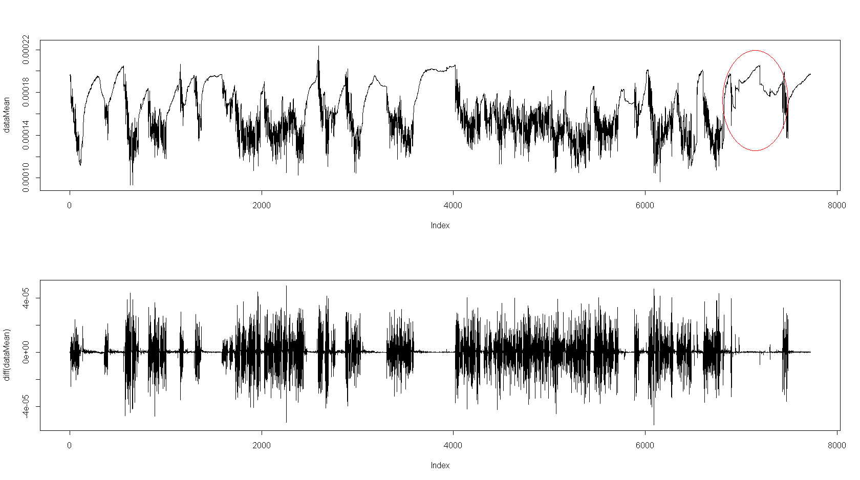
I've attached a picture of the time series I'm talking about. The top is the original series, the bottom is the differenced series.

Each data point is a 5 minute average reading from a strain gauge. This strain gauge is placed on a machine. The noisy areas correspond to areas where the machine is turned on, the clean areas are when the machine is turned off. If you look at the area circled in red, there are anomalous steps in the reading that I would like to be able to detect automatically.

I'm completely stumped on how I might be able to do this - any ideas?

enter image description here

$\endgroup$
3
  • $\begingroup$ What is anomalous steps? is it the machine is turned off? I could see similar patten in red circle in the other part of series? Did I miss something to see in the plot? $\endgroup$
    – vinux
    Commented Jan 5, 2012 at 5:25
  • $\begingroup$ This seems difficult. My fisrt thought: model the (hidden) on/off state by a Markov Chain. The phenomenon you want to detect is a the occurence of a few important values in the differenced series when the machine is off, so if you can compute at each moment the probability for the machine to be off, you may be able detect it as "important values when the off probability is high". $\endgroup$
    – Elvis
    Commented Jan 5, 2012 at 7:10
  • $\begingroup$ I had a second thought. I’ll post it... $\endgroup$
    – Elvis
    Commented Jan 5, 2012 at 9:21

3 Answers 3

15
$\begingroup$

It appears you are looking for spikes within intervals of relative quiet. "Relative" means compared to typical nearby values, which suggests smoothing the series. A robust smooth is desirable precisely because it should not be influenced by a few local spikes. "Quiet" means variation around that smooth is small. Again, a robust estimate of local variation is desirable. Finally, a "spike" would be a large residual as a multiple of the local variation.

To implement this recipe, we need to choose (a) how close "nearby" means, (b) a recipe for smoothing, and (c) a recipe for finding local variation. You may have to experiment with (a), so let's make it an easily controllable parameter. Good, readily available choices for (b) and (c) are Lowess and the IQR, respectively. Here is an R implementation:

library(zoo)                      # For the local (moving window) IQR
f <- function(x, width=7) {       # width = size of moving window in time steps
    w <- width / length(x)
    y <- lowess(x, f=w)           # The smooth
    r <- zoo(x - y$y)             # Its residuals, structured for the next step
    z <- rollapply(r, width, IQR) # The running estimate of variability
    r/z                           # The diagnostic series: residuals scaled by IQRs
}

As an example of its use, consider these simulated data where two successive spikes are added to a quiet period (two in a row should be harder to detect than one isolated spike):

> x <- c(rnorm(192, mean=0, sd=1), rnorm(96, mean=0, sd=0.1), rnorm(192, mean=0, sd=1))
> x[240:241] <- c(1,-1) # Add a local spike
> plot(x)
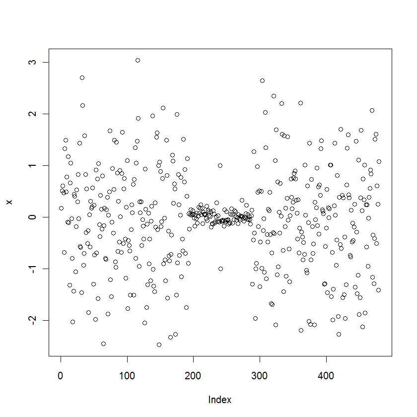
Simulated data

Here is the diagnostic plot:

> u <- f(x)
> plot(u)
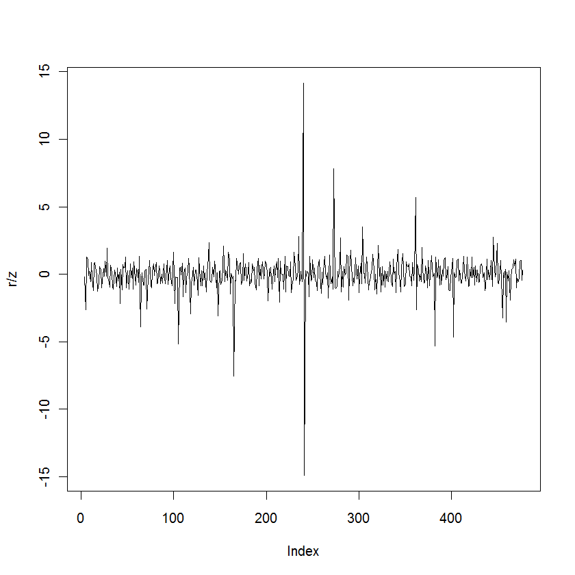
Diagnostic plot

Despite all the noise in the original data, this plot beautifully detects the (relatively small) spikes in the center. Automate the detection by scanning f(x) for largish values (larger than about 5 in absolute value: experiment to see what works best with sample data).

> spikes <- u[abs(u) >= 5]
      240       241       273 
 9.274959 -9.586756  6.319956

The spurious detection at time 273 was a random local outlier. You can refine the test to exclude (most) such spurious values by modifying f to look for simultaneously high values of the diagnostic r/z and low values of the running IQR, z. However, although the diagnostic has a universal (unitless) scale and interpretation, the meaning of a "low" IQR depends on the units of the data and has to be determined from experience.
$\endgroup$
4
  • $\begingroup$ The last paragraph was based on simulated data much like, but not exactly the same as, those shown here. In this diagnostic plot it is clear there are other spurious values up to about 7.5 in size and the two spikes have values around 14. $\endgroup$
    – whuber
    Commented Jan 5, 2012 at 15:27
  • $\begingroup$ Nice answer - this looks promising. Thanks a lot. I'll get back to you later with my results. $\endgroup$ Commented Jan 5, 2012 at 21:34
  • $\begingroup$ Just a quick follow up - I did a similar thing to what you did, but I had access to the standard deviation of the data within each data point (ie. within each 5 min period). I divided by the smoothed STD and I got some pretty good results. $\endgroup$ Commented Jan 10, 2012 at 22:09
  • $\begingroup$ wow, I missed that! (+1!) $\endgroup$
    – Elvis
    Commented Jan 14, 2012 at 13:37
3
$\begingroup$

Here is a two cents suggestion.

Denote $X_t$ the differenced series. Given $\Delta > 0$ and a point $t$, define $$a(\Delta,t) = {1\over 2\Delta + 1} |X_t|.$$

For let’s says $\Delta = 50$, the value of $a(\Delta,t)$ characterizes the off/on zones by low/high values.

An anomalous step is a point $t$ where $|X_t| > \alpha a(\Delta,t)$ – you’ll need to do some tuning on $\alpha, \Delta$ to detect what you want, and avoid false positive when the machine turns on. I’d try first with $\Delta = 50$ and $\alpha = 4$.

Alternatively, you can look at points $t$ where $a(\delta,t) > \alpha a(\Delta,t)$ for a $\delta\ll\Delta$ (eg $\delta = 10$, $\Delta = 100$), that may help the fine tuning (in that case, you would take a smaller value for $\alpha$).

$\endgroup$
1
  • $\begingroup$ is it possible to write an R code to implement this? Thanks! $\endgroup$
    – user9292
    Commented Jul 27, 2012 at 17:23
0
$\begingroup$

If you actually know the machine state - on or off, this is an important input and can be solved as a regression model, or more specifically a control model.

I don't know much about strain models, but the curves remind me of some of the physical models for circuits, like the Hodgkin Huxley equations. Or more generally, you can estimate the first order differential equation by regressing the $Y_i$ on the $X_i$, $X_{i-1}$, and $Y_{i-1}$ where $X_i$ is the machine state at time $i$ (on, off) and $Y_i$ is the amplitude (or whatever) on your y-axis in the graph of the time series.

With a known physical model, you can calculate the residuals, and easily use clustering or other methods to identify these abnormal periods. For instance, a simple boxcar filter can be used to identify segments of time where the average residual exceeds a certain threshold, identified using classifier development techniques.

$\endgroup$

Your Answer

By clicking “Post Your Answer”, you agree to our terms of service and acknowledge you have read our privacy policy.

Not the answer you're looking for? Browse other questions tagged or ask your own question.