normal approximation to the binomial distribution: why np>5?

Question

Nearly every text book which discusses the normal approximation to the binomial distribution mentions the rule of thumb that the approximation can be used if $np\geq5$ and $n(1-p)\geq 5$. Some books suggest $np(1-p)\geq 5$ instead. The same constant $5$ often shows up in discussions of when to merge cells in the $\chi^2$-test. None of the texts I found gives a justification or reference for this rule of thumb.

Where does this constant 5 come from? Why not 4 or 6 or 10? Where was this rule of thumb originally introduced?

Answer 1

Some possibilities are offered by the Wikipedia article on the Binomial distribution, under the section on Normal approximation, which currently includes the following comment (emphasis mine):

Another commonly used rule is that both values $np$ and $n(1-p)$ must be greater than 5. However, the specific number varies from source to source, and depends on how good an approximation one wants.

Now there, this is associated with ensuring that the normal approximation $x\sim N(\mu,\sigma)$ falls within the legal bounds for a binomial variable, $x\in[0,n]$.

To spell this out, if we parameterize the desired coverage probability in terms of a z-score $z>0$, then we have $$ \mu \pm z\sigma \in [0,n] \implies z\sigma \leq \min[\,\mu \,,\, n - \mu \,] \implies z^2 \leq \min\left[\,\tfrac{\mu^2}{\sigma^2} \,,\, \tfrac{(n - \mu)^2}{\sigma^2}\,\right] $$ Using the Binomial moments $\mu=np$ and $\sigma^2=np(1-p)$, the above constraints require $$\min\!\big[\,p\,,1-p\,\big]n \geq z^2$$ So for this approach $z^2=5$ would correspond to a coverage probability of $$\Phi[\sqrt{5}\,]-\Phi[-\sqrt{5}\,]\approx 97.5\%$$ where $\Phi$ is the standard normal CDF.

So to the extent this coverage probability is "pretty" and 5 is a nice round number ... that could give some justification perhaps? I do not have much experience with probability texts, so cannot say how common "5" is, vs. other "specific numbers" to use the phrasing of Wikipedia. My feeling is there is nothing really special about 5, and Wikipedia suggests 9 is common also (corresponding to a "pretty" $z$ of 3).

Answer 2

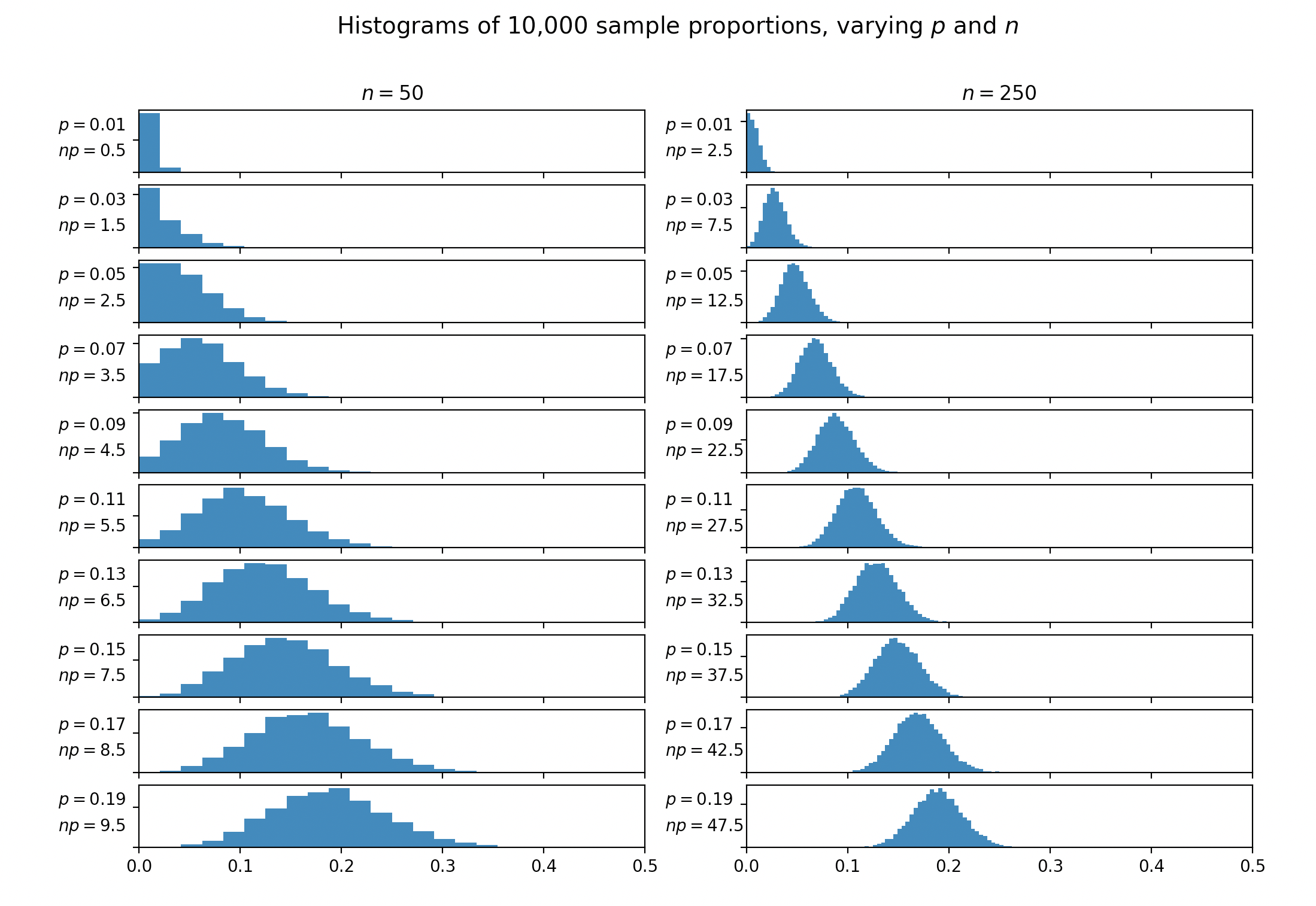
In addition to the excellent answers already posted, I thought it might be helpful to have a visualization exploring the distributions of observed proportions for varying $n$ and $p$ values.

To generate the below histograms, I took $n$ samples from a Bernoulli trial with probability $p$, and repeated this process 10,000 times. I then generated a histogram of the observed proportions from each of those 10,000 experiments.

Visually speaking, it looks like $np \geq 5$ is fairly reasonable. Although when $n=50$ there does seem to still be some clipping going on with $np = 5.5$ and $np = 6.5$. Once you get to $np = 7.5$, the impact seems pretty small.

Also note that these plots would be symmetrical for if we took new $p'$ values of $p' = (1 - p)$.

Python code to generate the plots. You can use this to tweak $n$ and $p$ if you want to experiment yourself.

import matplotlib.pyplot as plt
import numpy as np
np.random.seed(20190915)


def make_hists(axs, n):
    proportions = np.linspace(0.01, 0.19, len(axs))
    for i, prop in enumerate(proportions):
        # Draw n samples 10,000 times
        x = np.random.rand(n, 10_000) < prop
        means = x.mean(axis=0)
        axs[i].hist(means, bins=np.linspace(0, 0.5, n//2))
        axs[i].set_xlim([0, 0.5])
        axs[i].set_yticklabels([])
        ylim_mean = np.mean(axs[i].get_ylim())
        axs[i].text(-0.08, ylim_mean * 3/2, f'$p={prop:.2f}$', va='center')
        axs[i].text(-0.08, ylim_mean * 2/3, f'$np={n * prop:.1f}$', va='center')
    axs[0].set_title(f'$n={n}$')

def main():
    f, axs = plt.subplots(10, 2, sharex=True, figsize=(12, 8))
    make_hists(axs[:, 0], 50)
    make_hists(axs[:, 1], 250)
    f.suptitle(
        'Histograms of 10,000 sample proportions, varying $p$ and $n$',
        fontsize=14
    )
    plt.show()

main()

Answer 3

Not a complete explanation, but it's interesting to go back to Cochran 1952 Annals of Math Stats "The $\chi^2$ test of goodness of fit" (http://www.jstor.org/stable/2236678), Part II ("Some Aspects of the Practical Use of the Test"), which is of pretty respectable antiquity in the field ... Cochran discusses the history of the theoretical underpinnings of the test (Pearson 1900, Fisher 1922, 1924), but doesn't touch on the rule of thumb until the following passage ... [emphasis added]

7. The minimum expectation. Since x2 has been established as the limiting distribution of X2 in large samples, it is customary to recommend, in applications of the test, that the smallest expected number in any class should be 10 or (with some writers) 5. ... This topic has recently been subject to vigorous discussion among the psychologists [17], [18]. The numbers 10 and 5 appear to have been arbitrarily chosen. A few investigations throw some light on the appropriateness of the rule. The approach has been to examine the exact distribution of X2, when some or all expectations are small, either by mathematical methods or from sampling experiments.

The investigations are scanty and narrow in scope, as is to be expected since work of this type is time-consuming. Thus the recommendations given below may require modification when new evidence becomes available.

To digress for a moment, the problem of investigating the behavior of X2 when expectations are small is an example of a whole class of problems that are relevant to applied statistics. In applications it is an everyday occurrence to use the results of a body of theory in situations where we know, or strongly suspect, that some of the assumptions in the theory are invalid. Thus the literature contains investigations of the t-distribution when the parent population is nonnormal, and of the performance of linear regression estimates when the regression in the population is actually nonlinear. Fortunately for applications, the results of theory sometimes remain substantially true even when some assumptions fail to hold. This fact tends to make statistics a more confusing subject than pure mathematics, in which a result is usually either right or wrong.

As a personal note, I have often noticed a dilution effect in such rules of thumb, usually in the direction of permissiveness. Cochran says the rule is "10 (or sometimes 5)"; I think I've always seen it quoted as 5 (as in the OP). A similar process appears with the rules of thumb for number of observations required per parameter in regression models; Harrell's Regression Modeling Strategies quotes 10-20 but the lower value is almost always used in justifications ...

Answer 4

To fill in some details for the answer by @GeoMatt22:

Consider a binomial random variable with parameters $n$ and $p$, so that its mean $\mu=np$ and its variance $\sigma^2=np(1-p)$. For a number $z$ we have $$\mu \pm z\sigma \in [0,n] \iff 0\le \mu-z\sigma\le \mu+z\sigma\le n$$ $$ \iff z\sigma \leq \min[\,\mu \,,\, n - \mu \,] \iff z^2 \leq \min\left[\,\tfrac{\mu^2}{\sigma^2} \,,\, \tfrac{(n - \mu)^2}{\sigma^2}\,\right] $$ $$ \iff z^2 \le \min\left[\frac{n^2p^2}{np(1-p)}, \frac{(n-np)^2}{np(1-p)}\right] = n\min\left[\frac{p}{(1-p)}, \frac{(1-p)}{p}\right]. $$

Lemma: Let $p$ be a real number with $0< p< 1$. Then $$ \min\!\big[\,p\,,1-p\,\big] < \min\left[\frac{p}{1-p}, \frac{1-p}{p}\right] \le 2\cdot \min\!\big[\,p\,,1-p\,\big] $$

Proof: By symmetry, we may assume $p\le 1-p$. Then we must show: $ p < \frac{p}{1-p} \le 2 p . $ Multiplying by $\frac{1-p}p$, it is equivalent that $ (1-p)< 1 \le 2(1-p), $ which follows from $0<p\le 1/2$. []

By the lemma, $$z^2/n\le \min(p,1-p) \implies \mu\pm z\sigma\in [0,n] \implies z^2/n\le 2\min(p,1-p)$$

Suppose now that we are approximating the binomial with a normal $W$ with the same mean $\mu$ and standard deviation $\sigma$.

The condition that $np\ge 10$ and $n(1-p)\ge 10$ is equivalent to $n\min(p,1-p)\ge 10$.

If that holds then $$z^2\le 10 \implies z^2/n\le \min(p,1-p) \implies \mu\pm z\sigma\in [0,n]. $$ Let $Z=(W-\mu)/\sigma$. Then $$ 99.84\%=\mathbb P(|Z|\le \sqrt{10})\le \mathbb P(\mu \pm Z\sigma \in [0,n]). $$ Thus $n$ is large enough that an outcome chosen according to the normal distribution will fall inside $[0,n]$ with exceedingly large probability.

Answer 5

The rule provides a criteria that makes sure that p is neither close to 0 nor to 1. If it is closer to 0 or 1, the resulting distribution will not be a good apporximation to normal distribution.

You can see a pictorial justification of the same here