Convergence to zero of a sum involving the median

Question

Let $\{X_i:i=1,...,n\}$ be a sequence of i.i.d random variables with a continuous density function. If $m$ is the true median and $\hat m _n$ is the sample median, is it true that: $$\frac{\sum_{i=1}^{n}\big(1\{X_i\leq m\} - 1\{X_i\leq\hat m _n\}\big)}{\sqrt{n}}$$

goes to 0 in probability under suitable conditions?

Answer 1

Let's begin by parsing the meaning of the indicators.

1. $I\{X_i \le m\}$ is a random variable equal to $1$ when $X_i$ is at the (true) median $m$ or lower. Thus, by definition, it is a Bernoulli (that is, $0-1$) variable. All we need to know about it is the chance it equals $1$. Writing $F$ for the distribution of (any of the) $X_i$, that chance is $p=F(m)$.

2. $I\{X_i \le \hat m_n\}$ is a random variable equal to $1$ when $X_i$ is at the sample median $\hat m_n$ or lower. By definition, at least half of the sample is equal to or less than the sample median (and at least half is equal to or greater than the sample median).

We all know the difficulties with sample medians: they are uniquely defined only for samples whose size $n$ is odd and, when $F$ has a finite jump (reflecting one or more values with positive probabilities), there is some chance that several $X_i$ will be tied at the median value. A rigorous analysis would address these separate possibilities. To get some insight into how it might go, consider the simplest case where (a) $F$ has no finite jumps (this includes all continuous distributions) and (b) $n=2k+1$ is odd. Because of (a), it is certain there will be no tie at the median and because of (b), exactly $k+1$ of the $X_i$ (for $i$ ranging from $1$ through $n$) are equal to or less than the sample median. In this situation, then,

$$\sum_{i=1}^n I\{X_i \le \hat m_n\}$$

is a sum of $k+1$ ones and $k$ zeros, therefore equal to a constant $k+1$.

At this point, the rest is easy: the numerator of the fraction, being a sum of $n$ iid Bernoulli variables, has a Binomial$(p, n)$ distribution minus the constant $k+1$. Because $F$ has no jumps, $p=F(m)=1/2$. Therefore the numerator is a random variable with mean $p n = (2k+1)/2 = k+1/2$ minus $k+1$: its mean is $-1/2$. It variance is that of the Binomial$(p,n)$ distribution, equal to $p(1-p)n = 1/2(1-1/2)(n) = n/4$. The denominator divides the mean by $\sqrt{n}$ and causes the variance to be divided by $\sqrt{n}^2=n$. Consequently,

$$Z_n = \frac{\sum_{i=1}^{n}\big(1\{X_i\leq m\} - 1\{X_i\leq\hat m _n\}\big)}{\sqrt{n}}$$

is a random variable with mean $-1/(2\sqrt{n})$ and variance $1/4$. In fact, as is well known (it's an easy consequence of the Central Limit Theorem), the subsequence $Z_1, Z_3, \ldots, Z_{2k+1}, \ldots$ converges to a Normal distribution of mean zero and variance $1/4$. Because this is far from zero, the original sequence cannot possibly converge to zero.

---

It is actually more interesting when $F$ has a jump at its median. Specifically, this is the case where

$$F(m) = \Pr(X_i \le m) \gt 1/2 \text{ and } \Pr(X_i \ge m) \gt 1/2.$$

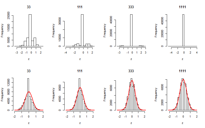
For very large $n$, the Central Limit Theorem implies the chance that $\hat m_n \ne m$ is vanishingly small (this chance rapidly decreases with $n$). Consequently, since $Z_n$ obviously is zero when $m=\hat m_n$, $Z_n$ will almost always equal zero. The limit in probability of the $Z_n$ must be zero in this case.

---

The two situations are readily simulated. The top row of the figure shows the cases where $F$ jumps at the median while the bottom row shows the continuous case. The headings give the sample sizes $n$. From left to right it is evident how the top row progresses toward a zero distribution while the bottom row progresses to a Normal distribution (whose density is shown as a red curve for reference).

Here is the R code that produced the figure.

n.sim <- 5e4 # Simulation size
k <- 4       # Jump of size k/(2k+1) in the middle of the distribution
n.size <- c(33, 111, 333, 1111) # Sample sizes
par(mfrow=c(2,length(n.size)))
for (n in n.size) {
  x <- matrix(floor(runif(n*n.sim, 0, 2*k+1)), nrow=n)
  z <- apply(x, 2, function(y) {sum(y <= k) - sum(y <= median(y))})/sqrt(n)
  hist(z, main=paste(n), freq=TRUE)
}
for (n in n.size) {
  x <- matrix(rnorm(n*n.sim, k), nrow=n)
  z <- apply(x, 2, function(y) {sum(y <= k) - sum(y <= median(y))})/sqrt(n)
  h <- hist(z, main=paste(n), freq=TRUE, breaks=25)
  dx <- diff(h$breaks[1:2])
  curve(dnorm(x, 0, 1/2)*n.sim*dx, add=TRUE, col="Red", lwd=2)
}