Test if multiple random variables have the same mean

Question

I am given an estimate of the mean and the variance of the estimated mean to 5 normally distributed random variables. I need to test if all 5 variables have the same mean.

When I look for an answer online I’m led to a single-sample ANOVA, but I cannot implement the ANOVA, because I don’t have sample data. I’ve thought about generating a sample that has the same mean and variance I’ve been given, but then it is unclear to me what to choose as the sample size; I could have a near infinite sample size and I don’t know how that affects the ANOVA calculations.

What I have done is calculate the pair wise difference distribution between all means and determined if this difference was some alpha value away from zero.

Does anyone know a test that compares multiple means simultaneously and that doesn’t require sample data?

Answer 1

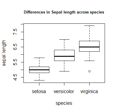
The one-way ANOVA calculated from summary statistics, can be followed with an example (in R). We can look at differences in sepal length between three species of Iris, comparing the output of the "manual" code with the built-in output for the ANOVA table.

We are looking at these differences:

The SUMMARY STATISTICS (including the number of specimens) are as follows:

# Number of specimens per species:
(n           = tapply(iris$Sepal.Length, iris$Species, length))
#    setosa versicolor  virginica 
#        50         50         50 
# Mean sepal length for each species:
(group_means = tapply(iris$Sepal.Length, iris$Species, mean))
#    setosa versicolor  virginica 
#     5.006      5.936      6.588 
# Sample variance of the sepal length for each species:
(group_var   = tapply(iris$Sepal.Length, iris$Species, var))
#    setosa versicolor  virginica 
#    0.1242490  0.2664327  0.4043429 

Now, working with these summary statistics we can calculate...

The variability between groups:

# First we need to calculate the overall mean:
grand_mean  = sum(n * group_means) / sum(n) 
#... to calculate the sum of square differences between groups:
(SS_between  = sum(n * (group_means - grand_mean)^2))
# [1] 63.21213
# with the corresponding degrees of freedom:
(df_between  = length(unique(iris$Species)) - 1)
# [1] 2
# and the mean square error:
(MS_between  = SS_between / df_between)
# [1] 31.60607

Now we can calculate the variability within groups:

It's worth at this point remembering that the sample variance is calculated as $s^2=\frac{\sum (x_i - \bar x )^2}{n-1}$ so that the $\displaystyle \text{SS}_{\text{within groups}}= \sum_{\text{groups}}(n-1) s^2.$

# We obtained the sum of squares within adding the numerators of the var's):
(SS_within   = sum((n - 1) * group_var))
# [1] 38.9562
# And calculate the degrees of freedom:
(df_within   = sum(n - 1))
# [1] 147
# And the mean squared error:
(MS_within   = SS_within / df_within)
# [1] 0.2650082

We calculate the F value and the p value as:

# The ratio of mean squared errors:
(F_value = MS_between / MS_within)
# [1] 119.2645
# and the corresponding probability:
(p_value = pf(F_value, df_between, df_within, lower.tail = F))
# [1] 1.669669e-31

Now we can compare these values to the output in R using the original dataset:

> anova(lm(iris$Sepal.Length ~ iris$Species))
Analysis of Variance Table

Response: iris$Sepal.Length
              Df Sum Sq Mean Sq F value    Pr(>F)    
iris$Species   2 63.212  31.606  119.26 < 2.2e-16 ***
Residuals    147 38.956   0.265           

Finally,

> (SS_total = SS_between + SS_within)
[1] 102.1683
> (df       = df_between + df_within)
[1] 149

---

After the comment to the initial answer by wherestheforce, I played a bit with carrying out the one-way ANOVA from summary statistics without knowing the group size. The assumption I made is that all the groups (categories) are the same size. The toy data is again the Iris dataset.

In the following ad hoc function, we run ANOVAS on randomly generated normal draws from the means and SDs in the problem. In each iteration, and starting at 2, we increase the group size up to a maximum group size we fix as input, $n.$ Each time we save the p value.

anv = function(means, sd, n){
  p.values = numeric(n) 
  for(i in 2:n){
    sam = data.frame(val = rnorm(i * length(means), 
                  rep(means, each = i), rep(sd, each = i)), 
                  group = factor(rep(1:length(means), each=i)))
    p = anova(lm(val ~ group, sam))$"Pr(>F)"[1]
    p.values[i] = p
  }
  (p.values = p.values[-1])
}

In the problem case in the Iris dataset, we have the following means and standard distributions:

> (group_means = tapply(iris$Sepal.Length, iris$Species, mean))
    setosa versicolor  virginica 
     5.006      5.936      6.588 
> (group_sd   = tapply(iris$Sepal.Length, iris$Species, sd))
    setosa versicolor  virginica 
 0.3524897  0.5161711  0.6358796 

and I'll smooth out asymptotic values by averaging across multiple replications of this Monte Carlo, for instance, 20 times:

anvs = rowMeans(replicate(20, anv(group_means, group_sd, 10)))

yielding values below p < 0.05 with $n$ values as low as $3:$

> (sig.group.size = which(anvs < 0.05) + 1)
[1]  3  4  5  6  7  8  9 10

Part of the OP...

it is unclear to me what to choose as the sample size; I could have a near infinite sample size and I don’t know how that affects the ANOVA calculations.

seems answered in the log-plot of the p values as the group size increases: